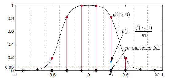
In this study, we present an efficient and novel unconditionally stable Monte Carlo simulation (MCS) for solving the multi-dimensional Allen–Cahn (AC) equation, which can model the motion by mean curvature flow of a hypersurface. We use an operator splitting method, where the diffusion and nonlinear terms are solved separately. The diffusion term is calculated using MCS for the stochastic differential equation, while the nonlinear term is locally computed for each particle in a virtual grid. Several numerical experiments are presented to demonstrate the performance of the proposed algorithm. The computational results confirm that the proposed algorithm can solve the AC equation more efficiently as the dimension of space increases.
Citation: Youngjin Hwang, Ildoo Kim, Soobin Kwak, Seokjun Ham, Sangkwon Kim, Junseok Kim. Unconditionally stable monte carlo simulation for solving the multi-dimensional Allen–Cahn equation[J]. Electronic Research Archive, 2023, 31(8): 5104-5123. doi: 10.3934/era.2023261
In this study, we present an efficient and novel unconditionally stable Monte Carlo simulation (MCS) for solving the multi-dimensional Allen–Cahn (AC) equation, which can model the motion by mean curvature flow of a hypersurface. We use an operator splitting method, where the diffusion and nonlinear terms are solved separately. The diffusion term is calculated using MCS for the stochastic differential equation, while the nonlinear term is locally computed for each particle in a virtual grid. Several numerical experiments are presented to demonstrate the performance of the proposed algorithm. The computational results confirm that the proposed algorithm can solve the AC equation more efficiently as the dimension of space increases.

| [1] |
S. M. Allen, J. W. Cahn, A microscopic theory for antiphase boundary motion and its application to antiphase domain coarsening, Acta Metall., 27 (1979), 1085–1095. https://doi.org/10.1016/0001-6160(79)90196-2 doi: 10.1016/0001-6160(79)90196-2

|
| [2] |
M. Olshanskii, X. Xu, V. Yushutin, A finite element method for Allen–Cahn equation on deforming surface, Comput. Math. Appl., 90 (2021), 148–158. https://doi.org/10.1016/j.camwa.2021.03.018 doi: 10.1016/j.camwa.2021.03.018
|
| [3] |
J. W. Choi, H. G. Lee, D. Jeong, J. Kim, An unconditionally gradient stable numerical method for solving the Allen–Cahn equation, Physica A, 388 (2009), 1791–1803. https://doi.org/10.1016/j.physa.2009.01.026 doi: 10.1016/j.physa.2009.01.026
|
| [4] |
Y. Li, H. G. Lee, D. Jeong, J. Kim, An unconditionally stable hybrid numerical method for solving the Allen–Cahn equation, Comput. Math. Appl., 60 (2010), 1591–1606. https://doi.org/10.1016/j.camwa.2010.06.041 doi: 10.1016/j.camwa.2010.06.041
|
| [5] |
H. D. Vuijk, J. M. Brader, A. Sharma, Effect of anisotropic diffusion on spinodal decomposition, Soft Matter, 15 (2019), 1319–1326. https://doi.org/10.1039/C8SM02017E doi: 10.1039/C8SM02017E
|
| [6] |
T. H. Fan, J. Q. Li, B. Minatovicz, E. Soha, L. Sun, S. Patel, et al., Phase-field modeling of freeze concentration of protein solutions, Polymers, 11 (2018), 10. https://doi.org/10.3390/polym11010010 doi: 10.3390/polym11010010
|
| [7] |
R. B. Marimont, M. B. Shapiro, Nearest neighbour searches and the curse of dimensionality, IMA J. Appl. Math., 24 (1979), 59–70. https://doi.org/10.1093/imamat/24.1.59 doi: 10.1093/imamat/24.1.59
|
| [8] |
X. Fang, L. Qiao, F. Zhang, F. Sun, Explore deep network for a class of fractional partial differential equations, Chaos Solitons Fractals, 172 (2023), 113528. https://doi.org/10.1016/j.chaos.2023.113528 doi: 10.1016/j.chaos.2023.113528
|
| [9] |
V. Charles, J. Aparicio, J. Zhu, The curse of dimensionality of decision-making units: A simple approach to increase the discriminatory power of data envelopment analysis, Eur. J. Oper. Res., 279 (2019), 929–940. https://doi.org/10.1016/j.ejor.2019.06.025 doi: 10.1016/j.ejor.2019.06.025
|
| [10] |
V. Berisha, C. Krantsevich, P. R. Hahn, S. Hahn, G. Dasarathy, P. Turaga, et al., Digital medicine and the curse of dimensionality, npj Digit. Med., 4 (2021), 153. https://doi.org/10.1038/s41746-021-00521-5 doi: 10.1038/s41746-021-00521-5
|
| [11] |
S. Koohy, G. Yao, K. Rubasinghe, Numerical solutions to low and high-dimensional Allen–Cahn equations using stochastic differential equations and neural networks, Partial Differ. Equations Appl. Math, 7 (2023), 100499. https://doi.org/10.1016/j.padiff.2023.100499 doi: 10.1016/j.padiff.2023.100499
|
| [12] |
S. Ham, Y. Hwang, S. Kwak, J. Kim, Unconditionally stable second-order accurate scheme for a parabolic sine–Gordon equation, AIP Adv., 12 (2022), 025203. https://doi.org/10.1063/5.0081229 doi: 10.1063/5.0081229
|
| [13] |
S. Ayub, H. Affan, A. Shah, Comparison of operator splitting schemes for the numerical solution of the Allen–Cahn equation, AIP Adv., 9 (2019), 125202. https://doi.org/10.1063/1.5126651 doi: 10.1063/1.5126651
|
| [14] |
H. G. Lee, A second-order operator splitting Fourier spectral method for fractional-in-space reaction-diffusion equations, J. Comput. Appl. Math., 333 (2018), 395–403. https://doi.org/10.1016/j.cam.2017.09.007 doi: 10.1016/j.cam.2017.09.007
|
| [15] |
D. Jeong, J. Kim, An explicit hybrid finite difference scheme for the Allen–Cahn equation, J. Comput. Appl. Math., 340 (2018), 247–255. https://doi.org/10.1016/j.cam.2018.02.026 doi: 10.1016/j.cam.2018.02.026
|
| [16] |
X. Yang, Z. Yang, C. Zhang, Stochastic heat equation: Numerical positivity and almost surely exponential stability, Comput. Math. Appl., 119 (2022), 312–318. https://doi.org/10.1016/j.camwa.2022.05.031 doi: 10.1016/j.camwa.2022.05.031
|
| [17] |
Y. Sun, M. Kumar, Numerical solution of high dimensional stationary Fokker–Planck equations via tensor decomposition and Chebyshev spectral differentiation, Comput. Math. Appl., 67 (2014), 1960–1977. https://doi.org/10.1016/j.camwa.2014.04.017 doi: 10.1016/j.camwa.2014.04.017
|
| [18] |
S. Shrestha, Monte carlo method to solve diffusion equation and error analysis, J. Nepal Math. Soc., 4 (2021), 54–60. https://doi.org/10.3126/jnms.v4i1.37113 doi: 10.3126/jnms.v4i1.37113
|
| [19] |
A. Medved, R. Davis, P. A. Vasquez, Understanding fluid dynamics from Langevin and Fokker–Planck equations, Fluids, 5 (2020), 40. https://doi.org/10.3390/fluids5010040 doi: 10.3390/fluids5010040
|
| [20] |
H. Naeimi, F. Kowsary, Finite Volume Monte Carlo (FVMC) method for the analysis of conduction heat transfer, J. Braz. Soc. Mech. Sci. Eng., 41 (2019), 1–10. https://doi.org/10.1007/s40430-019-1762-3 doi: 10.1007/s40430-019-1762-3
|
| [21] | H. Naeimi, Monte carlo methods for heat transfer, Int. J. Math. Game Theory Algebra, 29 (2020), 113–170. |
| [22] | T. Nakagawa, A. Tanaka, On a Monte Carlo scheme for some linear stochastic partial differential equations, Monte Carlo Methods Appl., 27 (2021), 169–193. https://doi.org/10.1515/mcma-2021-2088 |
| [23] |
G. Venkiteswaran, M. Junk, Quasi-Monte Carlo algorithms for diffusion equations in high dimensions, Monte Carlo Methods Appl., 68 (2005), 23–41. https://doi.org/10.1016/j.matcom.2004.09.003 doi: 10.1016/j.matcom.2004.09.003
|
| [24] | A. Novikov, D. Kuzmin, O. Ahmadi, Random walk methods for Monte Carlo simulations of Brownian diffusion on a sphere, Appl. Math. Comput., 364, (2020), 124670. https://doi.org/10.1016/j.amc.2019.124670 |
| [25] |
D. Lee, The numerical solutions for the energy-dissipative and mass-conservative Allen–Cahn equation, Comput. Math. Appl., 80 (2020), 263–284. https://doi.org/10.1016/j.camwa.2020.04.007 doi: 10.1016/j.camwa.2020.04.007
|
| [26] |
H. G. Lee, J. Y. Lee, A second order operator splitting method for Allen–Cahn type equations with nonlinear source terms, Physica A, 432 (2015), 24–34. https://doi.org/10.1016/j.physa.2015.03.012 doi: 10.1016/j.physa.2015.03.012
|
| [27] |
Y. Cheng, A. Kurganov, Z. Qu, T. Tang, Fast and stable explicit operator splitting methods for phase-field models, J. Comput. Phys., 303 (2015), 45–65. https://doi.org/10.1016/j.jcp.2015.09.005 doi: 10.1016/j.jcp.2015.09.005
|
| [28] |
A. Chertock, C. R. Doering, E. Kashdan, A. Kurganov, A fast explicit operator splitting method for passive scalar advection, J. Sci. Comput., 45 (2010), 200–214. https://doi.org/10.1007/s10915-010-9381-2 doi: 10.1007/s10915-010-9381-2
|
| [29] |
K. Poochinapan, B. Wongsaijai, Numerical analysis for solving Allen–Cahn equation in 1D and 2D based on higher-order compact structure-preserving difference scheme, Appl. Math. Comput., 434 (2022), 127374. https://doi.org/10.1016/j.amc.2022.127374 doi: 10.1016/j.amc.2022.127374
|
| [30] |
J. Kai, S. Wei, High-order energy stable schemes of incommensurate phase-field crystal model, Electron. Res. Arch., 28 (2020), 1077–1093. https://doi.org/10.3934/era.2020059 doi: 10.3934/era.2020059
|
| [31] |
W. Liupeng, H. Yunqing, Error estimates for second-order SAV finite element method to phase field crystal model, Electron. Res. Arch., 29 (2021), 1735–1752. https://doi.org/10.3934/era.2020089 doi: 10.3934/era.2020089
|
| [32] |
J. W. Choi, H. G. Lee, D. Jeong, J. Kim, An unconditionally gradient stable numerical method for solving the Allen–Cahn equation, Physica A, 388 (2009), 1791–1803. https://doi.org/10.1016/j.physa.2009.01.026 doi: 10.1016/j.physa.2009.01.026
|
| [33] | M. Franken, M. Rumpf, B. Wirth, A phase field based PDE constraint optimization approach to time discrete Willmore flow, Int. J. Numer. Anal. Model., 2011 (2011). |
| [34] | X. Chen, C. M. Elliott, A. Gardiner, J. JING ZHAO, Convergence of numerical solutions to the Allen–Cahn equation, Appl. Anal., 69 (1998), 47–56. |
| [35] | G. B. Folland, Introduction to Partial Differential Equations, Princeton university press, 1976. https://doi.org/10.1515/9780691213033 |
| [36] |
R. A. Fisher, The wave of advance of advantageous genes, Ann. Eugen., 7 (1937), 355–369. https://doi.org/10.1111/j.1469-1809.1937.tb02153.x doi: 10.1111/j.1469-1809.1937.tb02153.x
|
| [37] | A. Kolmogorov, Étude de l'équation de la diffusion avec croissance de la quantité de matière et son application à un problème biologique, Moscow Univ. Bull. Math., 1 (1937), 1–25. |
| [38] |
P. Román-Román, F. Torres-Ruiz, Modelling logistic growth by a new diffusion process: application to biological systems, Biosystems, 110 (2012), 9–21. https://doi.org/10.1016/j.biosystems.2012.06.004 doi: 10.1016/j.biosystems.2012.06.004
|
| [39] |
X. Y. Wang, Exact and explicit solitary wave solutions for the generalised fisher equation, Phys. Lett. A, 131 (1988), 277–279. https://doi.org/10.1016/0375-9601(88)90027-8 doi: 10.1016/0375-9601(88)90027-8
|


Figures(11) / Tables(3)
Youngjin Hwang, Ildoo Kim, Soobin Kwak, Seokjun Ham, Sangkwon Kim, Junseok Kim. Unconditionally stable monte carlo simulation for solving the multi-dimensional Allen–Cahn equation[J]. Electronic Research Archive, 2023, 31(8): 5104-5123. doi: 10.3934/era.2023261


 DownLoad: