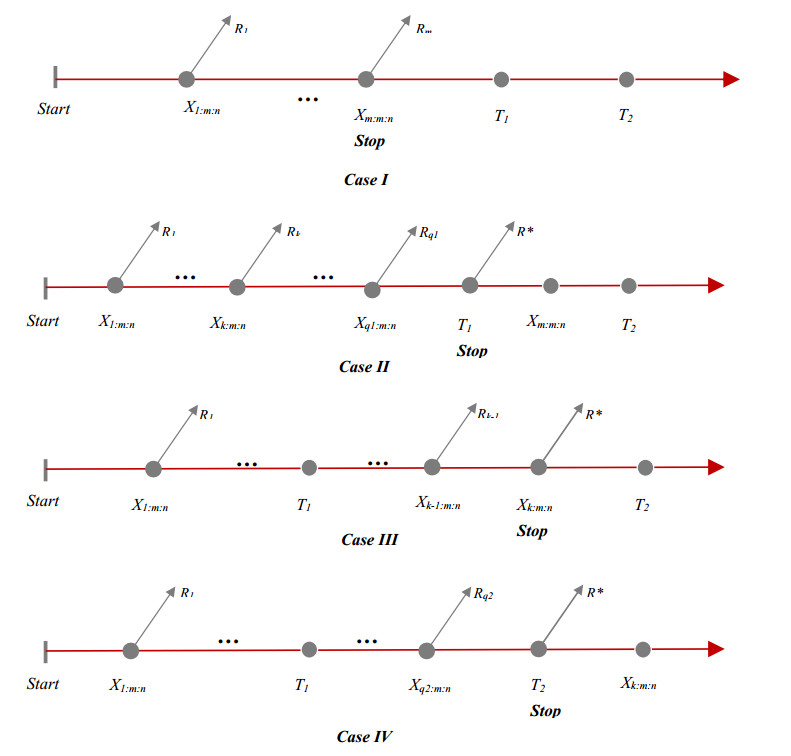
Censoring is a common occurrence in reliability engineering tests. This article considers estimation of the model parameters and the reliability characteristics of the gamma-mixed Rayleigh distribution based on a novel unified progressive hybrid censoring scheme (UPrgHyCS), where experimenters are allowed more flexibility in designing the test and higher efficiency. The maximum likelihood estimates of the model parameters and reliability are provided using the stochastic expectation–maximization algorithm based on the UPrgHyCS. Further, the Bayesian inference associated with any parametric function of the model parameters is considered using the Markov chain Monte Carlo method with the Metropolis-Hastings (M-H) algorithm. Asymptotic confidence and credible intervals of the proposed quantities are also created. The maximum a posteriori estimates of the model parameters are acquired. Due to the importance of determining the optimal censoring scheme for reliability problems, different optimality criteria are proposed and derived to find it. This method can help to design experiments and get more information about unknown parameters for a given sample size. Finally, comprehensive simulation experiments are provided to investigate the performances of the considered estimates, and a real dataset is analyzed to elucidate the practical application and the optimality criterion work in real life scenarios. The Bayes estimates using the M-H technique show the best performance in terms of error values.
Citation: Showkat Ahmad Lone, Hanieh Panahi, Sadia Anwar, Sana Shahab. Estimations and optimal censoring schemes for the unified progressive hybrid gamma-mixed Rayleigh distribution[J]. Electronic Research Archive, 2023, 31(8): 4729-4752. doi: 10.3934/era.2023242
Censoring is a common occurrence in reliability engineering tests. This article considers estimation of the model parameters and the reliability characteristics of the gamma-mixed Rayleigh distribution based on a novel unified progressive hybrid censoring scheme (UPrgHyCS), where experimenters are allowed more flexibility in designing the test and higher efficiency. The maximum likelihood estimates of the model parameters and reliability are provided using the stochastic expectation–maximization algorithm based on the UPrgHyCS. Further, the Bayesian inference associated with any parametric function of the model parameters is considered using the Markov chain Monte Carlo method with the Metropolis-Hastings (M-H) algorithm. Asymptotic confidence and credible intervals of the proposed quantities are also created. The maximum a posteriori estimates of the model parameters are acquired. Due to the importance of determining the optimal censoring scheme for reliability problems, different optimality criteria are proposed and derived to find it. This method can help to design experiments and get more information about unknown parameters for a given sample size. Finally, comprehensive simulation experiments are provided to investigate the performances of the considered estimates, and a real dataset is analyzed to elucidate the practical application and the optimality criterion work in real life scenarios. The Bayes estimates using the M-H technique show the best performance in terms of error values.

| [1] |
A. Childs, B. Chandrasekar, N. Balakrishnan, D. Kundu, Exact likelihood inference based on Type-Ⅰ and Type-Ⅱ hybrid censored samples from the exponential distribution, Ann. Inst. Stat. Math., 55 (2003), 319–330. https://doi.org/10.1007/BF02530502 doi: 10.1007/BF02530502

|
| [2] |
B. Chandrasekar, A. Childs, N. Balakrishnan, Exact likelihood inference for the exponential distribution under generalized Type-Ⅰ and Type-Ⅱ hybrid censoring, Nav. Res. Logis., 51(2004), 994–1004. https://doi.org/10.1002/nav.20038 doi: 10.1002/nav.20038
|
| [3] |
N. Balakrishnan, A. Rasouli, S. N. Farsipour, Exact likelihood inference based on an unified hybrid censored sample from the exponential distribution, J. Stat. Comput. Simul., 78 (2008), 475–488. https://doi.org/10.1080/00949650601158336 doi: 10.1080/00949650601158336
|
| [4] |
D. Kundu, H. Howlader, Bayesian inference and prediction of the inverse Weibull distribution for Type-Ⅱ censored data, Comput. Stat. Data Anal., 54 (2010), 1547–1558. https://doi.org/10.1016/j.csda.2010.01.003 doi: 10.1016/j.csda.2010.01.003
|
| [5] |
H. Panahi, Estimation of the Burr type Ⅲ distribution with application in unified hybrid censored sample of fracture toughness, J. Appl. Stat., 44 (2017), 2575–2592. https://doi.org/10.1080/02664763.2016.1258549 doi: 10.1080/02664763.2016.1258549
|
| [6] |
M. G. M. Ghazal, H. M. Hasaballah, Bayesian Prediction based on unified hybrid censored data from the exponentiated Rayleigh distribution, J. Stat. Appl. Probabil. Lett., 5 (2018), 103–118. https://doi.org/10.18576/jsapl/050301 doi: 10.18576/jsapl/050301
|
| [7] |
S. A. Lone, H. Panahi, Estimation procedures for partially accelerated life test model based on unified hybrid censored sample from the Gompertz distribution, Eksploat. i Niezawodn., 24 (2022), 427–436. https://doi.org/10.17531/ein.2022.3.4 doi: 10.17531/ein.2022.3.4
|
| [8] |
N. Balakrishnan, Progressive censoring methodology: An appraisal (with discussion), Test, 16 (2007), 211–296. https://doi.org/10.1007/s11749-007-0061-y doi: 10.1007/s11749-007-0061-y
|
| [9] |
T. Zhu, Z. Yan, X. Peng, A Weibull failure model to the study of the hierarchical Bayesian reliability, Eksploat. i Niezawodn., 18 (2016), 501–506. http://dx.doi.org/10.17531/ein.2016.4.4. doi: 10.17531/ein.2016.4.4
|
| [10] |
J. Gorny, E. Cramer, Modularization of hybrid censoring schemes and its application to unified progressive hybrid censoring, Metrika, 81 (2018), 173–210. https://doi.org/10.1007/s00184-017-0639-7 doi: 10.1007/s00184-017-0639-7
|
| [11] |
J. Kim, K. Lee, Estimation of the Weibull distribution under unified progressive hybrid censored data, J. Korean Data Anal. Soc., 20 (2018), 2189–2199. http://dx.doi.org/10.37727/jkdas.2018.20.5.2189 doi: 10.37727/jkdas.2018.20.5.2189
|
| [12] |
M. E. Ghitany, A compound Rayleigh survival model and its application to randomly censored data, Stat. Pap., 42 (2001), 437–450. https://doi.org/10.1007/s003620100072 doi: 10.1007/s003620100072
|
| [13] |
H. Panahi, N. Moradi, Estimation of the inverted exponentiated Rayleigh Distribution Based on Adaptive Type Ⅱ Progressive Hybrid Censored Sample, J. Comput. Appl. Math., 364 (2020), 112345. https://doi.org/10.1016/j.cam.2019.112345 doi: 10.1016/j.cam.2019.112345
|
| [14] |
W. K. Ghafi, T. J. Khraibet, A. A. Alwan, Maximum likelihood and Bayesian estimation of rayleigh with partly interval-censored case-Ⅰ data, NeuroQuantology, 18 (2020), 26–28. https://doi.org/10.14704/nq.2020.18.5.NQ20163 doi: 10.14704/nq.2020.18.5.NQ20163
|
| [15] |
S. Asadi, H. Panahi, C. Swarup, S. A. Lone, Inference on adaptive progressive hybrid censored accelerated life test for Gompertz distribution and its evaluation for virus-containing micro droplets data, Alex. Eng. J., 61 (2022), 10071–10084. https://doi.org/10.1016/j.aej.2022.02.061 doi: 10.1016/j.aej.2022.02.061
|
| [16] |
S. A. Lone, H. Panahi, I. Shah, Bayesian prediction interval for a constant-stress partially accelerated life test model under censored data, J. Taibah. Univ. Sci., 15 (2021), 1178–1187. https://doi.org/10.1080/16583655.2021.2023847 doi: 10.1080/16583655.2021.2023847
|
| [17] |
D. Kundu, B. Pradhan, Bayesian inference and life testing plans for generalized exponential distribution, Sci. China Ser. A.-Math., 52 (2009), 1373–1388. https://doi.org/10.1007/s11425-009-0085-8 doi: 10.1007/s11425-009-0085-8
|
| [18] |
L. L. Zhuang, A. Xu, X. L. Wang, A prognostic driven predictive maintenance framework based on Bayesian deep learning, Reliab. Eng. Syst. Safe., 234 (2023), 109181. https://doi.org/10.1016/j.ress.2023.10918 doi: 10.1016/j.ress.2023.10918
|
| [19] |
C. Luo, L. Shen, A. Xu, Modelling and estimation of system reliability under dynamic operating environments and lifetime ordering constraints, Reliab. Eng. Syst. Safe., 218 (2022), 108136. https://doi.org/10.1016/j.ress.2021.108136 doi: 10.1016/j.ress.2021.108136
|
| [20] |
S. Liu, W. Gui, Statistical inference for bathtub-shaped distribution based on generalized progressive hybrid censored data, Commun. Stat.-Theory Methods, 51 (2022), 8149–8172. https://doi.org/10.1080/03610926.2021.1889602 doi: 10.1080/03610926.2021.1889602
|
| [21] |
A. Xu, S. Zhou, Y. Tang, A unified model for system reliability evaluation under dynamic operating conditions, IEEE Trans. Reliab., 70 (2021), 65–72. https://doi.org/10.1109/TR.2019.2948173 doi: 10.1109/TR.2019.2948173
|
| [22] |
S. Park, N. Balakrishnan, S. W. Kim, Fisher information in progressive hybrid censoring schemes, Statistics, 45 (2011), 623–631. https://doi.org/10.1080/02331888.2010.504988 doi: 10.1080/02331888.2010.504988
|
| [23] |
A. P. Dempste, N. M. Laird, D. B. Rubin, Maximum likelihood from incomplete data via the EM algorithm, J. R. Stat. Soc. B: Stat. Methodol., 39 (1977), 1–38. https://doi.org/10.1111/j.2517-6161.1977.tb01600.x doi: 10.1111/j.2517-6161.1977.tb01600.x
|
| [24] |
T. R. Tsai, Y. Lio, W. C. Ting, EM Algorithm for Mixture Distributions Model with Type-Ⅰ Hybrid Censoring Scheme, Mathematics, 9 (2021), 2483. https://doi.org/10.3390/math9192483 doi: 10.3390/math9192483
|
| [25] |
L. A. Ferreira, J. L. Silva, Parameter estimation for Weibull distribution with right censored data using EM algorithm, Eksploat. i Niezawodn., 19 (2017), 310–315. https://doi.org/10.17531/ein.2017.2.20 doi: 10.17531/ein.2017.2.20
|
| [26] |
J. Diebolt, G. Celeux, Asymptotic properties of a stochastic EM algorithm for estimating mixing proportions, Commun. Stat. Stoch. Models, 9 (1993), 599–613. https://doi.org/10.1080/15326349308807283 doi: 10.1080/15326349308807283
|
| [27] |
M. Zhang, Z. Ye, M. Xie, A stochastic EM algorithm for progressively censored data analysis, Qual. Reliab. Eng. Int., 30 (2014), 711–722. https://doi.org/10.1002/qre.1522 doi: 10.1002/qre.1522
|
| [28] |
N. Metropolis, A. W. Rosenbluth, M. N. Rosenbluth, A. H. Teller, E. Teller, Equations of state calculations by fast computing machines, J. Chem. Phys., 21 (1953), 1087–1092. https://doi.org/10.1063/1.1699114 doi: 10.1063/1.1699114
|
| [29] |
W. K. Hastings, Monte Carlo sampling methods using Markov chains and their applications, Biometrika, 57 (1970), 97–109. https://doi.org/10.2307/2334940 doi: 10.2307/2334940
|
| [30] |
R. Di, P. Wang, C. He, Z. Guo, Constrained adjusted maximum a posteriori estimation of Bayesian network parameters, Entropy, 23 (2021), 1283. https://doi.org/10.3390/e23101283 doi: 10.3390/e23101283
|
| [31] | D. N. P. Murthy, M. Xie, R. Jiang, Weibull models, Wiley, New York, 2003. http://dx.doi.org/10.1002/047147326X |
| [32] | P. Congdon, Applied Bayesian Modelling, John Wiley & Sons, Chichester, 2014. |
Figures(8) / Tables(8)
Showkat Ahmad Lone, Hanieh Panahi, Sadia Anwar, Sana Shahab. Estimations and optimal censoring schemes for the unified progressive hybrid gamma-mixed Rayleigh distribution[J]. Electronic Research Archive, 2023, 31(8): 4729-4752. doi: 10.3934/era.2023242


 DownLoad: