Labor cost reduction and resourceful space utilization are essential for efficient warehouse operation. In these challenges, mobile rack technology can increase storage space by 75% or more. The mobile racking system is a system where racks are constructed on a mobile base and steered by rails on the floor. Driven by an electrical motor, the mobile base moves along the rails to open one or more access aisles. Moving rack technology eliminates aisle space between racks and increases storage space by synchronizing wheels or rails. Hence, companies can stock and access a high volume of products while enduring space-efficient. Minimizing the cost per pallet is especially critical for cooler and freezer facilities. However, there is no straightforward solution to determining the optimal layout of a mobile rack warehouse. When designing a mobile rack warehouse, you can increase storage space by a minimum of aisles, but it can reduce work efficiency at the same time. Therefore, it is necessary to determine the appropriate layout of mobile racks considering both work efficiency and space efficiency. This study proposes a practical layout of a mobile rack warehouse to harmonize work and space efficiency. To validate the model, we examine several numerical examples and analyze the warehouse area, the total amount of rack movement, and working hours. Depending on the operating cost, a different layout is suggested.
Citation: Dong Yun Shin, Jaeyoung Lee, Hyesung Seok. A study of layout determination of mobile rack warehouse[J]. AIMS Environmental Science, 2023, 10(4): 467-477. doi: 10.3934/environsci.2023026
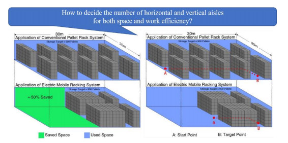
Labor cost reduction and resourceful space utilization are essential for efficient warehouse operation. In these challenges, mobile rack technology can increase storage space by 75% or more. The mobile racking system is a system where racks are constructed on a mobile base and steered by rails on the floor. Driven by an electrical motor, the mobile base moves along the rails to open one or more access aisles. Moving rack technology eliminates aisle space between racks and increases storage space by synchronizing wheels or rails. Hence, companies can stock and access a high volume of products while enduring space-efficient. Minimizing the cost per pallet is especially critical for cooler and freezer facilities. However, there is no straightforward solution to determining the optimal layout of a mobile rack warehouse. When designing a mobile rack warehouse, you can increase storage space by a minimum of aisles, but it can reduce work efficiency at the same time. Therefore, it is necessary to determine the appropriate layout of mobile racks considering both work efficiency and space efficiency. This study proposes a practical layout of a mobile rack warehouse to harmonize work and space efficiency. To validate the model, we examine several numerical examples and analyze the warehouse area, the total amount of rack movement, and working hours. Depending on the operating cost, a different layout is suggested.

| [1] | Lee JW (2015) East Asian Logistics Trends, 2015: 92–101. |
| [2] | Choi S H, Hong K M, Kim H J. (2018) A Study on Needs of the Logistics Technology in Korea, Korea Maritime Institute. |
| [3] | https://www.hankyung.com/news/article/2016102515801 |
| [4] | https://www.datexcorp.com/2022-warehousing-update-mobile-racking-systems/ |
| [5] | Lee M K (1995) Travel-Time Analysis for an Automated Mobile Racking System. J Korean Inst Ind Eng 21: 195–206. |
| [6] | Seila A F, Ceric V, Tadikamalla P R. Applied simulation modeling[M]. Duxbury Press, 2003. |
| [7] | Yun Y S, Seo S C, Lee S C (2000) Productivity Analysis of a Car Parts Assembly Line Using a 3D Simulation Tool. J Korean Inst Plant Eng 5. |
| [8] | Kim HS, Yoo SS, Cheon GM. (2016) A study on the multi-mobile rack work control algorithm. Proceedings of the Conference of the Korean Operations Research and Management Science Society 738–761. |
| [9] | Shin JY, Park HJ, Kim HS. (2016) Development of algorithm for optimum management using mobile-rack in distribution c enter. J Korean Soc Supply Chain Manag 16: 1–10. |
| [10] | Shin JY, Kim HS, Park HJ (2016) A study on an efficient cargo placement algorithm inside a mobile rack warehouse. Proceedings of the Spring Conference of the Korean Institute of Industrial Engineers 4493–4511. |
| [11] | https://www.jracking.com/mobile-racking-system/automatic-electric-mobile-pallet-rack.html |
| [12] | Manzini R (2006) Correlated storage assignment in an order picking system. Int J Ind Eng-theory 13 384–394. |
| [13] |
Boysen N, Briskorn D, Emde S (2017) Sequencing of picking orders in mobile rack warehouses. Eur J Oper Res 259: 293–307. https://doi.org/10.1016/j.ejor.2016.09.046 doi: 10.1016/j.ejor.2016.09.046

|
| [14] |
Boysen N, Briskorn D, Emde S (2017) Parts-to-picker based order processing in a rack-moving mobile robots environment. Eur J Oper Res 262: 550–562. https://doi.org/10.1016/j.ejor.2017.03.053 doi: 10.1016/j.ejor.2017.03.053
|
| [15] |
Lamballais T, Roy D, De Koster M B M. 2017. Estimating performance in a robotic mobile fulfillment system. Eur J Oper Res 256: 976–990. https://doi.org/10.1016/j.ejor.2016.06.063 doi: 10.1016/j.ejor.2016.06.063
|
| [16] | Zhang D, Si Y, Tian Z, et al. 2019. A Genetic-Algorithm Based Method for Storage Location Assignments in Mobile Rack Warehouses. In 2019 IEEE Global Communications Conference (GLOBECOM) (1–6). https://doi.org/10.1109/GLOBECOM38437.2019.9013447 |
| [17] |
Weidinger F, Boysen N, Briskorn D 2018. Storage assignment with rack-moving mobile robots in KIVA warehouses. Transport Sci 52: 1479–1495. https://doi.org/10.1287/trsc.2018.0826 doi: 10.1287/trsc.2018.0826
|
| [18] | Lee C K M, Lin B, Ng K K H, et al. (2019) Smart robotic mobile fulfillment system with dynamic conflict-free strategies considering cyber-physical integration. Advanced Engineering Informatics, 42, 100998. https://doi.org/10.1016/j.aei.2019.100998 |
| [19] |
da Costa Barros Í R, Nascimento T P (2021) Robotic Mobile Fulfillment Systems: A survey on recent developments and research opportunities. Robot Auton Syst 137: 103729. https://doi.org/10.1016/j.robot.2021.103729 doi: 10.1016/j.robot.2021.103729
|
| [20] |
Wang Z, Sheu J B, Teo C P, et al. (2021) Robot Scheduling for Mobile‐Rack Warehouses: Human–Robot Coordinated Order Picking Systems. Prod Oper Manag https://doi.org/10.1111/poms.13406 doi: 10.1111/poms.13406
|
| [21] | Wang Z, Xu W, Hu X, et al. (2021) Inventory allocation to robotic mobile-rack and picker-to-part warehouses at minimum order-splitting and replenishment costs. Ann Oper Res 1–25. https://doi.org/10.1007/s10479-021-04190-1 |
| [22] |
Foroughi A, Boysen N, Emde S, et al. (2021) High-density storage with mobile racks: Picker routing and product location. J Oper Res Soc 72: 535–553. https://doi.org/10.1080/01605682.2019.1700180 doi: 10.1080/01605682.2019.1700180
|
| [23] |
De Koster R, Le-Duc T, Roodbergen K J. 2007. Design and control of warehouse order picking: a literature review. Eur J Oper Res 182: 481–501. https://doi.org/10.1016/j.ejor.2006.07.009 doi: 10.1016/j.ejor.2006.07.009
|
| [24] |
Gu J, Goetschalckx M, McGinnis L F. 2007. Research on warehouse operation: a comprehensive review. Eur J Oper Res 177: 1–21. https://doi.org/10.1016/j.ejor.2006.02.025 doi: 10.1016/j.ejor.2006.02.025
|
| [25] | Jeong D, Seo Y. 2018. Golden section search and hybrid tabu search-simulated annealing for layout design of unequal-sized facilities with fixed input and output points. Int J Ind Eng 25. |
| [26] | Hwang H S, Cho G S 2003. A performance analysis of transporters for order picking warehouse design. Int J Ind Eng-Theory Appl Pract 10: 614–620. |
| [27] | Baek J K, Shin H J 2009. A simulation for warehouse traffic using ARENA. Korean Manag Consult Rev 9: 95–108. |
| [28] |
Baek J K, Shin H J. 2013. A simulation for warehouse considering traffic. J Korea Soc Simul 22: 119–128. https://doi.org/10.9709/JKSS.2013.22.4.119 doi: 10.9709/JKSS.2013.22.4.119
|


Figures(5) / Tables(1)

Dong Yun Shin, Jaeyoung Lee, Hyesung Seok. A study of layout determination of mobile rack warehouse[J]. AIMS Environmental Science, 2023, 10(4): 467-477. doi: 10.3934/environsci.2023026


 DownLoad: