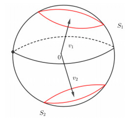
We study the energy of a ferromagnetic/antiferromagnetic frustrated spin system where the spin takes values on two disjoint circles of the 2-dimensional unit sphere. This analysis will be carried out first on a one-dimensional lattice and then on a two-dimensional lattice. The energy consists of the sum of a term that depends on nearest and next-to-nearest interactions and a penalizing term related to the spins' magnetic anisotropy transitions. We analyze the asymptotic behaviour of the energy, that is when the system is close to the helimagnet/ferromagnet transition point as the number of particles diverges. In the one-dimensional setting we compute the $ \Gamma $-limit of scalings of the energy at first and second order. As a result, it is shown how much energy the system spends for any magnetic anistropy transition and chirality transition. In the two-dimensional setting, by computing the $ \Gamma $-limit of a scaling of the energy, we study the geometric rigidity of chirality transitions.
Citation: Andrea Kubin, Lorenzo Lamberti. Variational analysis in one and two dimensions of a frustrated spin system: chirality and magnetic anisotropy transitions[J]. Mathematics in Engineering, 2023, 5(6): 1-37. doi: 10.3934/mine.2023094
We study the energy of a ferromagnetic/antiferromagnetic frustrated spin system where the spin takes values on two disjoint circles of the 2-dimensional unit sphere. This analysis will be carried out first on a one-dimensional lattice and then on a two-dimensional lattice. The energy consists of the sum of a term that depends on nearest and next-to-nearest interactions and a penalizing term related to the spins' magnetic anisotropy transitions. We analyze the asymptotic behaviour of the energy, that is when the system is close to the helimagnet/ferromagnet transition point as the number of particles diverges. In the one-dimensional setting we compute the $ \Gamma $-limit of scalings of the energy at first and second order. As a result, it is shown how much energy the system spends for any magnetic anistropy transition and chirality transition. In the two-dimensional setting, by computing the $ \Gamma $-limit of a scaling of the energy, we study the geometric rigidity of chirality transitions.

| [1] |
R. Alicandro, M. Cicalese, Variational analysis of the asymptotics of the XY model, Arch. Rational Mech. Anal., 192 (2009), 501–536. https://doi.org/10.1007/s00205-008-0146-0 doi: 10.1007/s00205-008-0146-0

|
| [2] |
R. Alicandro, M. Cicalese, A. Gloria, Variational description of bulk energies for bounded and unbounded spin systems, Nonlinearity, 21 (2008), 1881–1910. http://doi.org/10.1088/0951-7715/21/8/008 doi: 10.1088/0951-7715/21/8/008
|
| [3] | L. Ambrosio, N. Fusco, D. Pallara, Functions of bounded variation and free discontinuity problems, The Clarendon Press, 2000. |
| [4] |
A. Bach, M. Cicalese, L. Kreutz, G. Orlando, The antiferromagnetic $XY$ model on the triangular lattice: chirality transitions at the surface scaling, Calc. Var., 60 (2021), 149. https://doi.org/10.1007/s00526-021-02016-3 doi: 10.1007/s00526-021-02016-3
|
| [5] |
R. Badal, M. Cicalese, L. De Luca, M. Ponsiglione, $\Gamma$-convergence analysis of a generalized $XY$ model: fractional vortices and string defects, Commun. Math. Phys., 358 (2018), 705–739. https://doi.org/10.1007/s00220-017-3026-3 doi: 10.1007/s00220-017-3026-3
|
| [6] | A. Braides, $\Gamma$-convergence for beginners, Oxford: Oxford University Press, 2002. https://doi.org/10.1093/acprof: oso/9780198507840.001.0001 |
| [7] |
A. Braides, L. Truskinovsky, Asymptotic expansions by $\Gamma$-convergence, Continuum Mech. Thermodyn., 20 (2008), 21–62. https://doi.org/10.1007/s00161-008-0072-2 doi: 10.1007/s00161-008-0072-2
|
| [8] |
A. Braides, N. K. Yip, A quantitative description of mesh dependence for the discretization of singularly perturbed nonconvex problems, SIAM J. Numer. Anal., 50 (2012), 1883–1898. https://doi.org/10.1137/110822001 doi: 10.1137/110822001
|
| [9] |
M. Cicalese, M. Forster, G. Orlando, Variational analysis of a two-dimensional frustrated spin system: emergence and rigidity of chirality transitions, SIAM J. Math. Anal., 51 (2019), 4848–4893. https://doi.org/10.1137/19M1257305 doi: 10.1137/19M1257305
|
| [10] |
M. Cicalese, G. Orlando, M. Ruf, Emergence of concentration effects in the variational analysis of the $N$-clock model, Commun. Pure Appl. Anal., 75 (2019), 2279–2342. https://doi.org/10.1002/cpa.22033 doi: 10.1002/cpa.22033
|
| [11] |
M. Cicalese, M. Ruf, F. Solombrino, Chirality transitions in frustrated S$^2$-valued spin systems, Math. Mod. Meth. Appl. Sci., 26 (2016), 1481–1529. https://doi.org/10.1142/S0218202516500366 doi: 10.1142/S0218202516500366
|
| [12] |
M. Cicalese, F. Solombrino, Frustrated ferromagnetic spin chains: a variational approach to chirality transitions, J. Nonlinear Sci., 25 (2015), 291–313. https://doi.org/10.1007/s00332-015-9230-4 doi: 10.1007/s00332-015-9230-4
|
| [13] | H. T. Diep, Frustrated spin systems, World Scientific, 2005. https://doi.org/10.1142/5697 |
| [14] |
R. S. Dissanayaka Mudiyanselage, H. Wang, O. Vilella, M. Mourigal, G. Kotliar, W. Xie, LiYbSe2: Frustrated Magnetism in the Pyrochlore Lattice, J. Am. Chem. Soc., 144 (2022), 11933–11937. https://doi.org/10.1021/jacs.2c02839 doi: 10.1021/jacs.2c02839
|
| [15] |
D. V. Dmitriev, V. Ya Krivnov, Universal low-temperature properties of frustrated classical spin chain near the ferromagnet-helimagnet transition point, Eur. Phys. J. B, 82 (2011), 123–131. https://doi.org/10.1140/epjb/e2011-10664-6 doi: 10.1140/epjb/e2011-10664-6
|
| [16] |
S. L. Drechsler, O. Volkova, A. N. Vasiliev, N. Tristan, J. Richter, M. Schmitt, et al., Frustrated cuprate route from antiferromagnetic to ferromagnetic spin-$\frac12$ Heisenberg chains: Li$_{2}$ZrCuO$_{4}$ as a missing link near the quantum critical point, Phys. Rev. Lett., 98 (2007), 077202. https://doi.org/10.1103/PhysRevLett.98.077202 doi: 10.1103/PhysRevLett.98.077202
|
| [17] |
M. J. P. Gingras, P. A. McClarty, Quantum spin ice: a search for gapless quantum spin liquids in pyrochlore magnets, Rep. Prog. Phys., 77 (2014), 056501. https://doi.org/10.1088/0034-4885/77/5/056501 doi: 10.1088/0034-4885/77/5/056501
|
| [18] |
L. Modica, The gradient theory of phase transitions and the minimal interface criterion, Arch. Rational Mech. Anal., 98 (1987), 123–142. https://doi.org/10.1007/BF00251230 doi: 10.1007/BF00251230
|
| [19] | L. Modica, S. Mortola, Il limite nella $\Gamma$-convergenza di una famiglia di funzionali ellittici, (Italian), Boll. Un. Mat. Ital. A (5), 14 (1977), 526–529. |
| [20] |
D. G. Nocera, B. M. Bartlett, D. Grohol, D. Papoutsakis, M. P. Shores, Spin frustration in 2D kagomé lattices: a problem for inorganic synthetic chemistry, Chem.-Eur. J., 10 (2004), 3850–3859. https://doi.org/10.1002/chem.200306074 doi: 10.1002/chem.200306074
|
| [21] |
A. Poliakovsky, Upper bounds for singular perturbation problems involving gradient fields, J. Eur. Math. Soc., 9 (2007), 1–43. http://doi.org/10.4171/JEMS/70 doi: 10.4171/JEMS/70
|
| [22] |
K. Yu. Povarov, L. Facheris, S. Velja, D. Blosser, Z. Yan, S. Gvasaliya, et al., Magnetization plateaux cascade in the frustrated quantum antiferromagnet Cs$_2$CoBr$_4$, Phys. Rev. Res., 2 (2020), 043384. https://doi.org/10.1103/PhysRevResearch.2.043384 doi: 10.1103/PhysRevResearch.2.043384
|
| [23] | R. Skomski, Simple models of magnetism, Oxford University Press, 2008. https://doi.org/10.1093/acprof: oso/9780198570752.001.0001 |
| [24] |
R. Szymczak, P. Aleshkevych, C. P. Adams, S. N. Barilo, A. J. Berlinsky, J. P. Clancy, et al., Magnetic anisotropy in geometrically frustrated kagomé staircase lattices, J. Magn. Magn. Mater., 321 (2009), 793–795. https://doi.org/10.1016/j.jmmm.2008.11.076 doi: 10.1016/j.jmmm.2008.11.076
|

Figures(2)

Andrea Kubin, Lorenzo Lamberti. Variational analysis in one and two dimensions of a frustrated spin system: chirality and magnetic anisotropy transitions[J]. Mathematics in Engineering, 2023, 5(6): 1-37. doi: 10.3934/mine.2023094


 DownLoad: