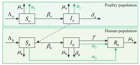
Avian influenza is an infectious viral disease caused by type A virus, which occurs frequently around the world and causes serious economic losses. Therefore, the adaptive control problem is explored in this paper for an avian influenza model in consideration of slaughtering to poultry, educational campaigns to the susceptible human and treatment to the infected human. First, by analyzing the transmission mechanism of avian influenza, a nonlinear adaptive control problem of avian influenza model is formulated, where some errors between model parameters and real values are allowed. Then, the parameters are estimated by constructing adaptive laws, which can be effectively used to design the applicative controllers to achieve the control goals. Besides, the stability of controlled model is analyzed with the aid of Lyapunov stability theory. Finally, numerical examples are proposed to verify the effectiveness and robustness of the designed controllers.
Citation: Ting Kang, Qimin Zhang, Qingyun Wang. Nonlinear adaptive control of avian influenza model with slaughter, educational campaigns and treatment[J]. Electronic Research Archive, 2023, 31(8): 4346-4361. doi: 10.3934/era.2023222
Avian influenza is an infectious viral disease caused by type A virus, which occurs frequently around the world and causes serious economic losses. Therefore, the adaptive control problem is explored in this paper for an avian influenza model in consideration of slaughtering to poultry, educational campaigns to the susceptible human and treatment to the infected human. First, by analyzing the transmission mechanism of avian influenza, a nonlinear adaptive control problem of avian influenza model is formulated, where some errors between model parameters and real values are allowed. Then, the parameters are estimated by constructing adaptive laws, which can be effectively used to design the applicative controllers to achieve the control goals. Besides, the stability of controlled model is analyzed with the aid of Lyapunov stability theory. Finally, numerical examples are proposed to verify the effectiveness and robustness of the designed controllers.

| [1] | Centers for Disease Control and Prevention, Seasonal Influenza (flu), Technical report, 2012. Available from: https://www.cdc.gov/flu/. |
| [2] | Public Health Agency of Canada, Human Health Issues Related to Avian Influenza in Canada, Technical report, 2006. Available from: https://www.canada.ca/en/public-health/services/reports-publications/human-health-issues-related-avian-influenza.html. |
| [3] |
P. Chen, J. Xie, Q. Lin, L. Zhao, Y. Zhang, H. Chen, et al., A study of the relationship between human infection with avian influenza a (H5N6) and environmental avian influenza viruses in Fujian, China, BMC Infect. Dis., 19 (2019), 762. https://doi.org/10.1186/s12879-019-4145-6 doi: 10.1186/s12879-019-4145-6

|
| [4] |
H. Gao, H. Lu, B. Cao, B. Du, H. Shang, J. Gan, et al., Clinical findings in 111 cases of influenza A (H7N9) virus infection, N. Engl. J. Med., 368 (2013), 2277–2285. https://doi.org/10.1056/NEJMoa1305584 doi: 10.1056/NEJMoa1305584
|
| [5] |
R. Gao, B. Cao, Y. Hu, Z. Feng, D. Wang, W. Hu, et al., Human infection with a novel avian-origin influenza A (H7N9) virus, N. Engl. J. Med., 368 (2013), 1888–1897. https://doi.org/ 10.1056/NEJMoa1304459 doi: 10.1056/NEJMoa1304459
|
| [6] |
D. Liu, W. Shi, Y. Shi, D. Wang, H. Xiao, W. Li, et al., Origin and diversity of novel avian influenza A H7N9 viruses causing human infection: phylogenetic, structural, and coalescent analyses, Lancet, 381 (2013), 1926–1932. https://doi.org/10.1016/S0140-6736(13)60938-1 doi: 10.1016/S0140-6736(13)60938-1
|
| [7] |
E. Claas, A. Osterhaus, R. Van-Beek, J. Jong, G. F. Rimmelzwaan, D. A. Senne, et al., Human influenza A H5N1 virus related to a highly pathogenic avian influenza virus, Lancet, 351 (1998), 472–477. https://doi.org/10.1016/S0140-6736(97)11212-0 doi: 10.1016/S0140-6736(97)11212-0
|
| [8] |
T. Kang, Q. Zhang, L. Rong, A delayed avian influenza model with avian slaughter: stability analysis and optimal control, Physica A, 529 (2019), 121544. https://doi.org/10.1016/j.physa.2019.121544 doi: 10.1016/j.physa.2019.121544
|
| [9] |
K. A. Pawelek, A. Oeldorf-Hirsch, L. Rong, Modeling the impact of twitter on influenza epidemics, Math. Biosci. Eng., 11 (2014), 1337–1356. https://doi.org/10.3934/mbe.2014.11.1337 doi: 10.3934/mbe.2014.11.1337
|
| [10] | World Health Organization, Human infection with avian influenza A (H7N9) virus–update, 2014. Available from: https://www.who.int/emergencies/disease-outbreak-news/item/2014_09_04_avian_influenza-en. |
| [11] |
L. Chen, X. Lin, W. Guo, J. Tian, W. Wang, X. Ying, et al., Diversity and evolution of avian influenza viruses in live poultry markets, free-range poultry and wild wetland birds in China, J. Gen. Virol., 97 (2016), 844–854. https://doi.org/10.1099/jgv.0.000399 doi: 10.1099/jgv.0.000399
|
| [12] |
K. Shimizu, L. Wulandari, E. D. Poetranto, R. A. Setyoningrum, R. Yudhawati, A. Sholikhah, et al., Seroevidence for a high prevalence of subclinical infection with avian influenza A(H5N1) virus among workers in a livepoultry market in Indonesia, J. Infect. Dis., 214 (2016), 1929–1936. https://doi.org/10.1093/infdis/jiw478 doi: 10.1093/infdis/jiw478
|
| [13] |
C. Bao, L. Cui, M. Zhou, L. Hong, G. F. Gao, H. Wang, Live-animal markets and influenza A (H7N9) virus infection, N. Engl. J. Med., 368 (2013), 2337–2339. https://doi.org/10.1056/NEJMc1306100 doi: 10.1056/NEJMc1306100
|
| [14] |
Y. Xiao, X. Sun, S. Tang, J. Wu, Transmission potential of the novel avian influenza A(H7N9) infection in mainland China, J. Theor. Biol., 352 (2014), 1–5. https://doi.org/10.1016/j.jtbi.2014.02.038 doi: 10.1016/j.jtbi.2014.02.038
|
| [15] |
X. Wang, W. Cheng, Z. Yu, S. Liu, H. Mao, E. Chen, Risk factors for avian influenza virus in backyard poultry flocks and environments in Zhejiang province, China: a cross-sectional study, Infect. Dis. Poverty, 7 (2018), 65. https://doi.org/10.1186/s40249-018-0445-0 doi: 10.1186/s40249-018-0445-0
|
| [16] |
E. Jung, S. Iwami, Y. Takeuchi, T. Jo, Optimal control strategy for prevention of avian influenza pandemic, J. Theor. Biol., 260 (2009), 220–229. https://doi.org/10.1016/j.jtbi.2009.05.031 doi: 10.1016/j.jtbi.2009.05.031
|
| [17] |
T. Kang, Q. Zhang, H. Wang, Optimal control of an avian influenza model with multiple time delays in state and control variables, Discrete Contin. Dyn. Syst. - Ser. B, 26 (2021), 4147–4171. https://doi.org/10.3934/dcdsb.2020278 doi: 10.3934/dcdsb.2020278
|
| [18] |
S. Sharma, A. Mondal, A. Pal, G. P. Samanta, Stability analysis and optimal control of avian influenza virus A with time delays, Int. J. Dyn. Control, 6 (2018), 1351–1366. https://doi.org/10.1007/s40435-017-0379-6 doi: 10.1007/s40435-017-0379-6
|
| [19] |
B. Cao, X. Nie, Event-triggered adaptive neural networks control for fractional-order nonstrict-feedback nonlinear systems with unmodeled dynamics and input saturation, Neural Networks, 142 (2021), 288–302. https://doi.org/10.1016/j.neunet.2021.05.014 doi: 10.1016/j.neunet.2021.05.014
|
| [20] |
B. Cao, X. Nie, Z. Wu, C. Xue, J. Cao, Adaptive neural network control for nonstrict-feedback uncertain nonlinear systems with input delay and asymmetric time-varying state constraints, J. Franklin Inst., 358 (2021), 7073–7095. https://doi.org/10.1016/j.jfranklin.2021.07.020 doi: 10.1016/j.jfranklin.2021.07.020
|
| [21] |
B. Cao, T. Kang, Nonlinear adaptive control of COVID-19 with media campaigns and treatment, Biochem. Biophys. Res. Commun., 555 (2021), 202–209. https://doi.org/10.1016/j.bbrc.2020.12.105 doi: 10.1016/j.bbrc.2020.12.105
|
| [22] |
H. Moradi, M. Sharifi, G. Vossoughi, Adaptive robust control of cancer chemotherapy in the presence of parametric uncertainties: a comparison between three hypotheses, Comput. Biol. Med., 56 (2015), 145–157. https://doi.org/10.1016/j.compbiomed.2014.11.002 doi: 10.1016/j.compbiomed.2014.11.002
|
| [23] |
M. H. Nematollahi, R. Vatankhah, M. Sharifi, Nonlinear adaptive control of tuberculosis with consideration of the risk of endogenous reactivation and exogenous reinfection, J. Theor. Biol., 486 (2020), 110081. https://doi.org/10.1016/j.jtbi.2019.110081 doi: 10.1016/j.jtbi.2019.110081
|
| [24] |
Y. Hayama, Y. Kimura, T. Yamamoto, S. Kobayashi, T, Tsutsui, Potential risk associated with animal culling and disposal during the foot-and-mouth disease epidemic in Japan in 2010, Res. Vet. Sci., 102 (2015), 228–230. https://doi.org/10.1016/j.rvsc.2015.08.017 doi: 10.1016/j.rvsc.2015.08.017
|
| [25] |
B. Barnes, A. Scott, M. Hernandez-Jover, J. A. Toribio, B. Moloney, K. Glass, Modelling high pathogenic avian influenza outbreaks in the commercial poultry industry, Theor. Popul Biol., 126 (2019), 59–71. https://doi.org/10.1016/j.tpb.2019.02.004 doi: 10.1016/j.tpb.2019.02.004
|
| [26] |
A. Wang, Y. Xiao, A Filippov system describing media effects on the spread of infectious diseases, Nonlinear Anal. Hybrid Syst., 11 (2014), 84–97. https://doi.org/10.1016/j.nahs.2013.06.005 doi: 10.1016/j.nahs.2013.06.005
|
| [27] |
X. Zhang, X. Liu, Backward bifurcation of an epidemic model with saturated treatment function, J. Math. Anal. Appl., 348 (2008), 433–443. https://doi.org/10.1016/j.jmaa.2008.07.042 doi: 10.1016/j.jmaa.2008.07.042
|
| [28] | J. J. E. Slotine, W. Li, Applied Nonlinear Control, Prentice Hall, Englewood Cliffs, New Jersey, 1991. |
| [29] | F. Chen, J. Cui, Cross-species epidemic dynamic model of influenza, in 2016 9th International Congress on Image and Signal Processing, BioMedical Engineering and Informatics (CISP-BMEI), (2016), 1567–1572. https://doi.org/10.1109/CISP-BMEI.2016.7852965 |
| [30] |
S. Liu, S. Ruan, X. Zhang, Nonlinear dynamics of avian influenza epidemic models, Math. Biosci., 283 (2017), 118–135. https://doi.org/10.1016/j.mbs.2016.11.014 doi: 10.1016/j.mbs.2016.11.014
|
Figures(12) / Tables(1)
Ting Kang, Qimin Zhang, Qingyun Wang. Nonlinear adaptive control of avian influenza model with slaughter, educational campaigns and treatment[J]. Electronic Research Archive, 2023, 31(8): 4346-4361. doi: 10.3934/era.2023222


 DownLoad: