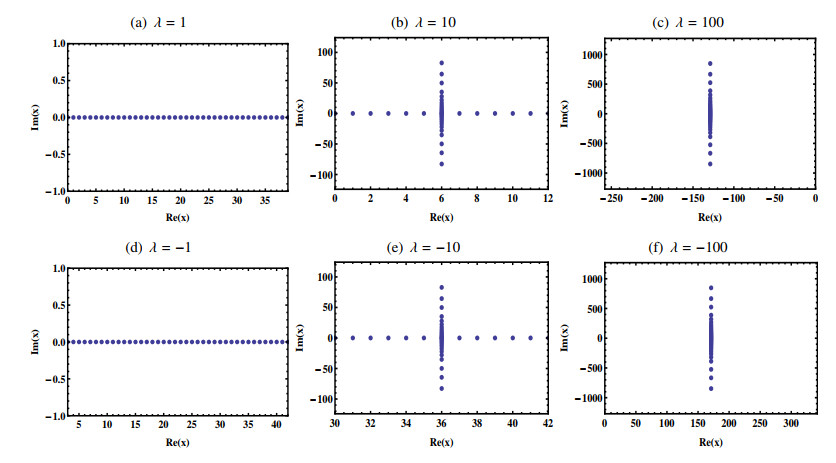
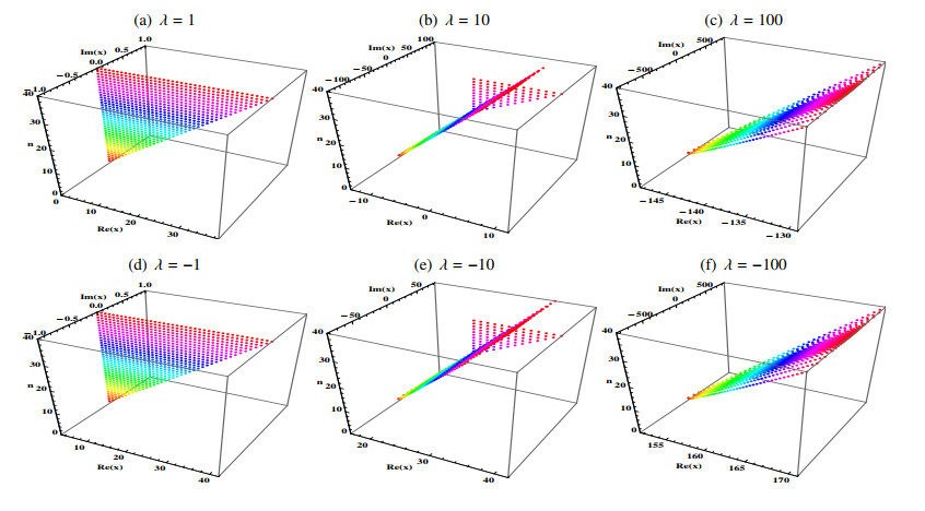
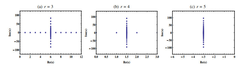
The degenerate versions of special polynomials and numbers, initiated by Carlitz, have regained the attention of some mathematicians by replacing the usual exponential function in the generating function of special polynomials with the degenerate exponential function. To study the relations between degenerate special polynomials, $ \lambda $-umbral calculus, an analogue of umbral calculus, is intensively applied to obtain related formulas for expressing one $ \lambda $-Sheffer polynomial in terms of other $ \lambda $-Sheffer polynomials. In this paper, we study the connection between degenerate higher-order Daehee polynomials and other degenerate type of special polynomials. We present explicit formulas for representations of the polynomials using $ \lambda $-umbral calculus and confirm the presented formulas between the degenerate higher-order Daehee polynomials and the degenerate Bernoulli polynomials, for example. Additionally, we investigate the pattern of the root distribution of these polynomials.
Citation: Dojin Kim, Sangbeom Park, Jongkyum Kwon. Some identities of degenerate higher-order Daehee polynomials based on $ \lambda $-umbral calculus[J]. Electronic Research Archive, 2023, 31(6): 3064-3085. doi: 10.3934/era.2023155
The degenerate versions of special polynomials and numbers, initiated by Carlitz, have regained the attention of some mathematicians by replacing the usual exponential function in the generating function of special polynomials with the degenerate exponential function. To study the relations between degenerate special polynomials, $ \lambda $-umbral calculus, an analogue of umbral calculus, is intensively applied to obtain related formulas for expressing one $ \lambda $-Sheffer polynomial in terms of other $ \lambda $-Sheffer polynomials. In this paper, we study the connection between degenerate higher-order Daehee polynomials and other degenerate type of special polynomials. We present explicit formulas for representations of the polynomials using $ \lambda $-umbral calculus and confirm the presented formulas between the degenerate higher-order Daehee polynomials and the degenerate Bernoulli polynomials, for example. Additionally, we investigate the pattern of the root distribution of these polynomials.

| [1] |
R. Dere, Y. Simsek, H. Srivastava, A unified presentation of three families of generalized Apostol type polynomials based upon the theory of the umbral calculus and the umbral algebra, J. Number Theory, 133 (2013), 3245–3263. https://doi.org/10.1016/j.jnt.2013.03.004 doi: 10.1016/j.jnt.2013.03.004

|
| [2] |
E. Doha, Y. Youssri, On the connection coefficients and recurrence relations arising from expansions in series of modified generalized Laguerre polynomials: Applications on a semi-infinite domain, Nonlinear Eng., 8 (2019), 318–327. https://doi.org/10.1515/nleng-2018-0073 doi: 10.1515/nleng-2018-0073
|
| [3] |
W. Abd-Elhameed, Y. Youssri, Solutions of the connection problems between Fermat and generalized Fibonacci polynomials, JP J. Algebra, Number Theory Appl., 38 (2016), 349–362. https://doi.org/10.17654/NT038040349 doi: 10.17654/NT038040349
|
| [4] | W. Abd-Elhameed, Y. Youssri, New connection formulae between Chebyshev and Lucas polynomials: New expressions involving Lucas numbers via hypergeometric functions, Adv. Stud. Contemp. Math., 28 (2018), 357–367. |
| [5] |
W. Abd-Elhameed, Y. Youssri, Connection formulae between generalized Lucas polynomials and some Jacobi polynomials: Application to certain types of fourth-order BVPs, Int. J. Appl. Comput. Math., 6 (2020), 45. https://doi.org/10.1007/s40819-020-0799-4 doi: 10.1007/s40819-020-0799-4
|
| [6] |
W. Abd-Elhameed, Y. Youssri, N. El-Sissi, M. Sadek, New hypergeometric connection formulae between Fibonacci and Chebyshev polynomials, Ramanujan J., 42 (2017), 347–361. https://doi.org/10.1007/s11139-015-9712-x doi: 10.1007/s11139-015-9712-x
|
| [7] | S. Roman, The Umbral Calculus, Academic Press, London, UK, 1984. |
| [8] |
T. Kim, D. S. Kim, Some identities on truncated polynomials associated with degenerate Bell polynomials, Russ. J. Math. Phys., 28 (2021), 342–355. https://doi.org/10.1134/S1061920821030079 doi: 10.1134/S1061920821030079
|
| [9] | T. K. Kim, D. S. Kim, H. I. Kwon, A note on degenerate stirling numbers and their applications, Proc. Jangjeon Math. Soc., 21 (2018), 195–203. |
| [10] |
T. Kim, D. Kim, H. Lee, J. Kwon, Representations by degenerate Daehee polynomials, Open Math., 20 (2022), 179–194. https://doi.org/10.1515/math-2022-0013 doi: 10.1515/math-2022-0013
|
| [11] |
J. Kwon, P. Wongsason, Y. Kim, D. Kim, Representations of modified type 2 degenerate poly-Bernoulli polynomials, AIMS Math., 7 (2022), 11443–11463. https://doi.org/10.3934/math.2022638 doi: 10.3934/math.2022638
|
| [12] |
L. Carlitz, A degenerate Staudt-Clausen theorem, Arch. Math., 7 (1956), 28–33. https://doi.org/10.1007/BF01900520 doi: 10.1007/BF01900520
|
| [13] |
D. S. Kim, T. Kim, Daehee numbers and polynomials, Appl. Math. Sci., 7 (2013), 5969–5976. https://doi.org/10.12988/ams.2013.39535 doi: 10.12988/ams.2013.39535
|
| [14] |
D. S. Kim, T. Kim, Degenerate Sheffer sequences and $\lambda$-Sheffer sequences, J. Math. Anal. Appl., 493 (2021), 124521. https://doi.org/10.1016/j.jmaa.2020.124521 doi: 10.1016/j.jmaa.2020.124521
|
| [15] |
T. Kim, D. S. Kim, H. Kim, J. Kwon, Some results on degenerate Daehee and Bernoulli numbers and polynomials, Adv. Differ. Equations, 2020 (2020), 1–13. https://doi.org/10.1186/s13662-020-02778-8 doi: 10.1186/s13662-020-02778-8
|
| [16] |
J. W. Park, J. Kwon, A note on the degenerate high order Daehee polynomials, Appl. Math. Sci., 9 (2015), 4635–4642. http://doi.org/10.12988/ams.2015.56416 doi: 10.12988/ams.2015.56416
|
| [17] |
D. S. Kim, T. Kim, A note on a new type of degenerate Bernoulli numbers, Russ. J. Math. Phys., 27 (2020), 227–235. https://doi.org/10.1134/S1061920820020090 doi: 10.1134/S1061920820020090
|
| [18] | T. Kim, A note on degenerate stirling polynomials of the second kind, arXiv preprint, (2017), arXiv: 1704.02290. https://doi.org/10.48550/arXiv.1704.02290 |
| [19] | J. Riordan, An Introduction to Combinatorial Analysis, Princeton University Press, 1958. |
| [20] |
T. Kim, D. S. Kim, H. K. Kim, H. Lee, Some properties on degenerate Fubini polynomials, Appl. Math. Sci. Eng., 30 (2022), 235–248. https://doi.org/10.1080/27690911.2022.2056169 doi: 10.1080/27690911.2022.2056169
|
| [21] | L. Carlitz, Degenerate Stirling, Bernoulli and Eulerian numbers, Util. Math., 15 (1979), 51–88. |
| [22] |
T. Kim, L. C. Jang, D. S. Kim, H. Y. Kim, Some identities on type 2 degenerate Bernoulli polynomials of the second kind, Symmetry, 12 (2020), 510. https://doi.org/10.3390/sym12040510 doi: 10.3390/sym12040510
|
| [23] | G. W. Jang, T. Kim, A note on type 2 degenerate Euler and Bernoulli polynomials, Adv. Stud. Contemp. Math., 29 (2019), 147–159. |
| [24] |
D. S. Kim, T. Kim, T. Mansour, J. J. Seo, Degenerate Mittag-Leffler polynomials, Appl. Math. Comput., 274 (2016), 258–266. https://doi.org/10.1016/j.amc.2015.11.014 doi: 10.1016/j.amc.2015.11.014
|
| [25] | N. Korobov, Special polynomials and their applications, Math. Notes, 2 (1996), 77–89. |
| [26] |
T. Kim, D. S. Kim, Degenerate polyexponential functions and degenerate Bell polynomials, J. Math. Anal. Appl., 487 (2020), 124017. https://doi.org/10.1016/j.jmaa.2020.124017 doi: 10.1016/j.jmaa.2020.124017
|
| [27] |
T. Kim, D. S. Kim, H. Y. Kim, J. Kwon, Some identities of degenerate Bell polynomials, Mathematics, 8 (2020), 40. https://doi.org/10.3390/math8010040 doi: 10.3390/math8010040
|

Figures(4)
Dojin Kim, Sangbeom Park, Jongkyum Kwon. Some identities of degenerate higher-order Daehee polynomials based on $ \lambda $-umbral calculus[J]. Electronic Research Archive, 2023, 31(6): 3064-3085. doi: 10.3934/era.2023155


 DownLoad: