Modeling and computation for unsteady blood flow and solute concentration in a constricted porous artery

Daniel N. Riahi; Saulo Orizaga; Daniel N. Riahi; Saulo Orizaga

doi:10.3934/bioeng.2023007

AIMS Bioengineering

2023, Volume 10, Issue 1: 67-88. doi: 10.3934/bioeng.2023007

Previous Article Next Article

Research article

Modeling and computation for unsteady blood flow and solute concentration in a constricted porous artery

Daniel N. Riahi ^1,2,
Saulo Orizaga ^{3
,
,}

1.
Department of Mechanical Science and Engineering, University of Illinois at Urbana-Champaign, Urbana, 61801, IL
2.
School of Mathematical & Statistical Sciences, University of Texas Rio Grande Valley, Brownsville, 78520, Texas
3.
Department of Mathematics, New Mexico Institute of Mining and Technology, Socorro, 87801, New Mexico

Received: 20 November 2022 Revised: 23 February 2023 Accepted: 24 February 2023 Published: 07 March 2023

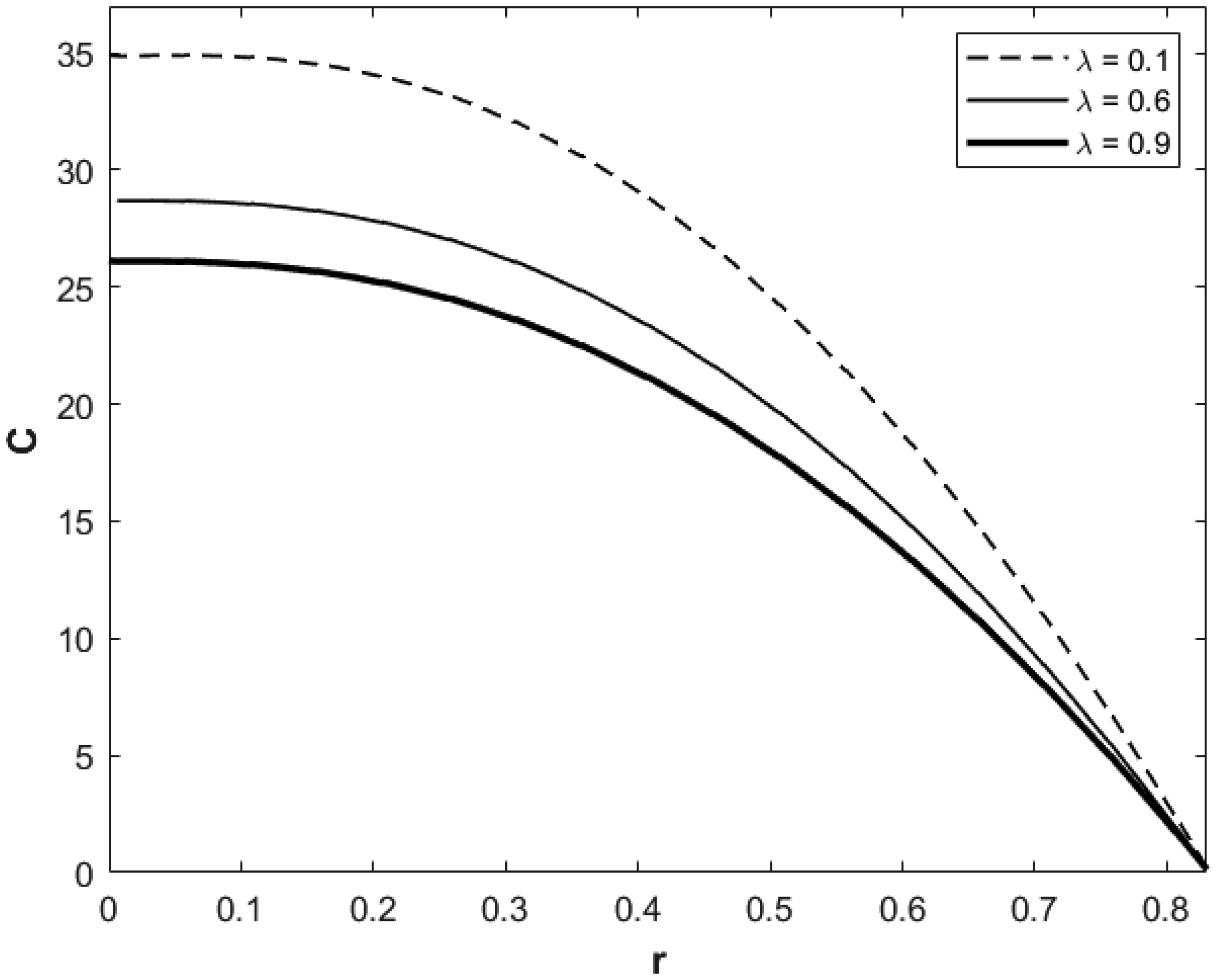
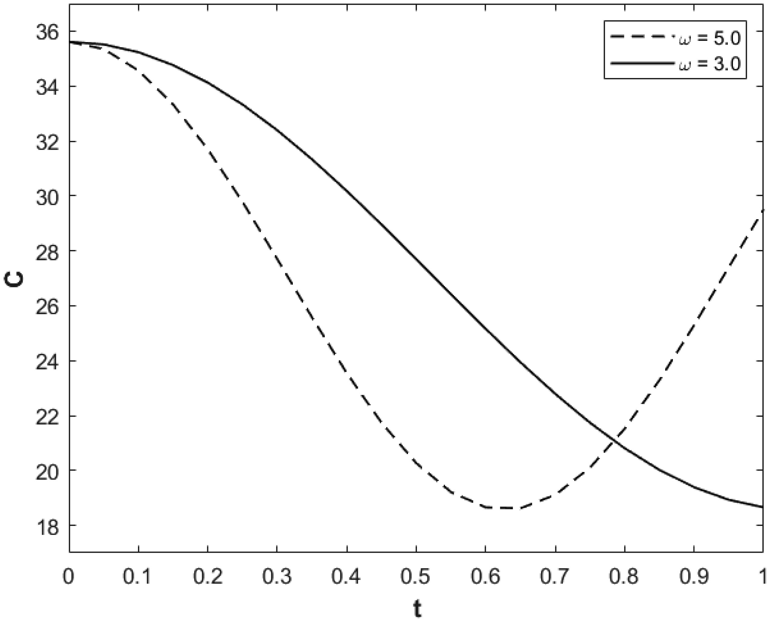
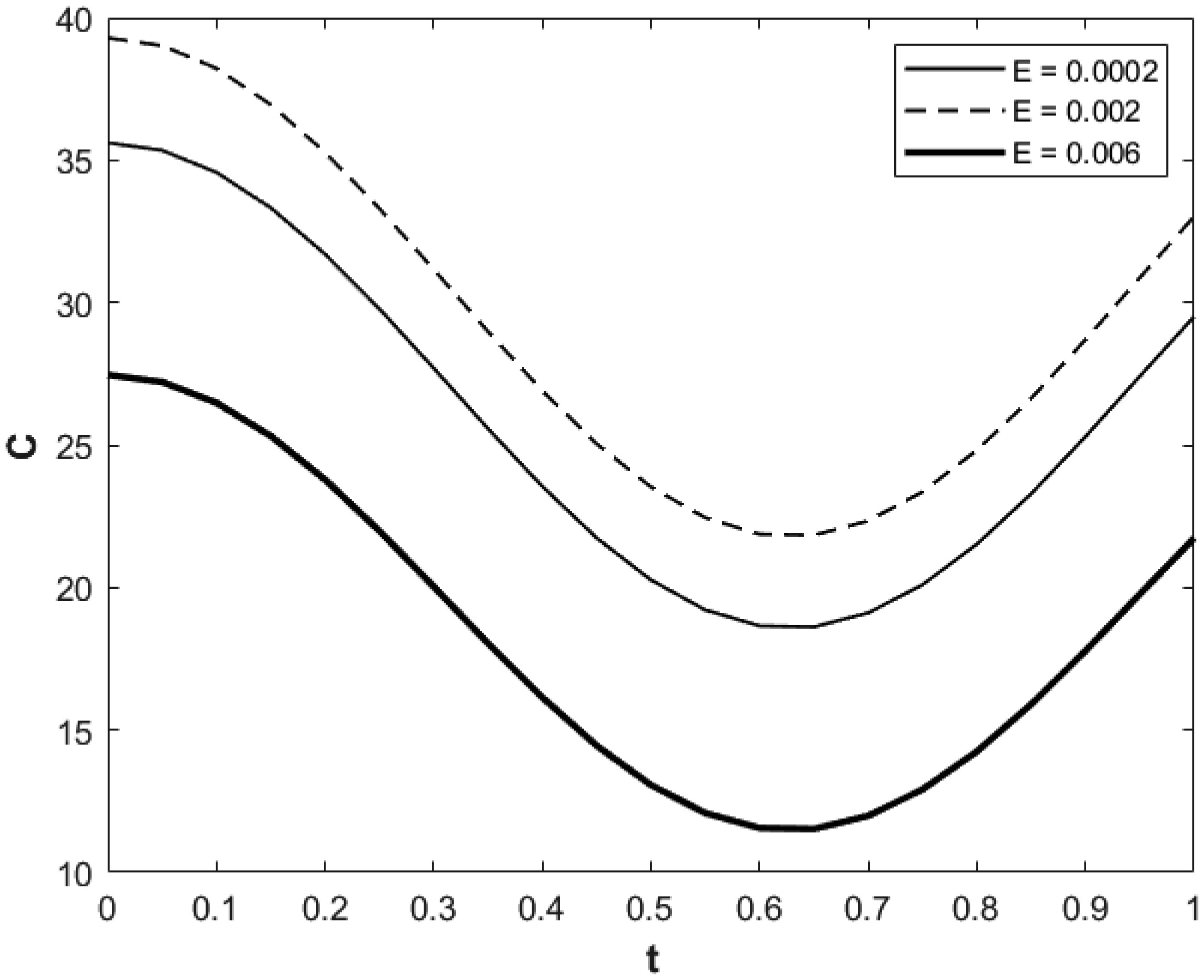
We investigated a physical system for unsteady blood flow and solute transport in a section of a constricted porous artery. The aim of this study was to determine effects of hematocrit, stenosis, pulse oscillation, diffusion, convection and chemical reaction on the solute transport. The significance of this study was uncovering combined roles played by stenosis height, hematocrit, pulse oscillation period, reactive rate, blood speed, blood pressure force and radial and axial extent of the porous artery on the solute transported by the blood flow in the described porous artery. We used both analytical and computational methods to determine blood flow quantities and solute transport for different parametric values of the described physical system. We found that solute transport increases with increasing stenosis height, blood pulsation period, convection and blood pressure force. However, transportation of solute reduces with increasing hematocrit, chemical reactive rate and radial or axial distance.

Keywords:

Citation: Daniel N. Riahi, Saulo Orizaga. Modeling and computation for unsteady blood flow and solute concentration in a constricted porous artery[J]. AIMS Bioengineering, 2023, 10(1): 67-88. doi: 10.3934/bioeng.2023007

Related Papers:

[1]	Jing Zhang, Baoqun Yin, Yu Zhong, Qiang Wei, Jia Zhao, Hazrat Bilal . A two-stage grasp detection method for sequential robotic grasping in stacking scenarios. Mathematical Biosciences and Engineering, 2024, 21(2): 3448-3472. doi: 10.3934/mbe.2024152
[2]	Xuewu Wang, Bin Tang, Xin Zhou, Xingsheng Gu . Double-robot obstacle avoidance path optimization for welding process. Mathematical Biosciences and Engineering, 2019, 16(5): 5697-5708. doi: 10.3934/mbe.2019284
[3]	Ruiping Yuan, Jiangtao Dou, Juntao Li, Wei Wang, Yingfan Jiang . Multi-robot task allocation in e-commerce RMFS based on deep reinforcement learning. Mathematical Biosciences and Engineering, 2023, 20(2): 1903-1918. doi: 10.3934/mbe.2023087
[4]	Zhen Yang, Junli Li, Liwei Yang, Qian Wang, Ping Li, Guofeng Xia . Path planning and collision avoidance methods for distributed multi-robot systems in complex dynamic environments. Mathematical Biosciences and Engineering, 2023, 20(1): 145-178. doi: 10.3934/mbe.2023008
[5]	Chengjun Wang, Xingyu Yao, Fan Ding, Zhipeng Yu . A trajectory planning method for a casting sorting robotic arm based on a nature-inspired Genghis Khan shark optimized algorithm. Mathematical Biosciences and Engineering, 2024, 21(2): 3364-3390. doi: 10.3934/mbe.2024149
[6]	Baoye Song, Shumin Tang, Yao Li . A new path planning strategy integrating improved ACO and DWA algorithms for mobile robots in dynamic environments. Mathematical Biosciences and Engineering, 2024, 21(2): 2189-2211. doi: 10.3934/mbe.2024096
[7]	Liwei Yang, Lixia Fu, Ping Li, Jianlin Mao, Ning Guo, Linghao Du . LF-ACO: an effective formation path planning for multi-mobile robot. Mathematical Biosciences and Engineering, 2022, 19(1): 225-252. doi: 10.3934/mbe.2022012
[8]	Ping Li, Liwei Yang . Conflict-free and energy-efficient path planning for multi-robots based on priority free ant colony optimization. Mathematical Biosciences and Engineering, 2023, 20(2): 3528-3565. doi: 10.3934/mbe.2023165
[9]	Xinyu Shao, Zhen Liu, Baoping Jiang . Sliding-mode controller synthesis of robotic manipulator based on a new modified reaching law. Mathematical Biosciences and Engineering, 2022, 19(6): 6362-6378. doi: 10.3934/mbe.2022298
[10]	Xingjia Li, Jinan Gu, Zedong Huang, Chen Ji, Shixi Tang . Hierarchical multiloop MPC scheme for robot manipulators with nonlinear disturbance observer. Mathematical Biosciences and Engineering, 2022, 19(12): 12601-12616. doi: 10.3934/mbe.2022588

Abstract

Abbreviations

L₀:

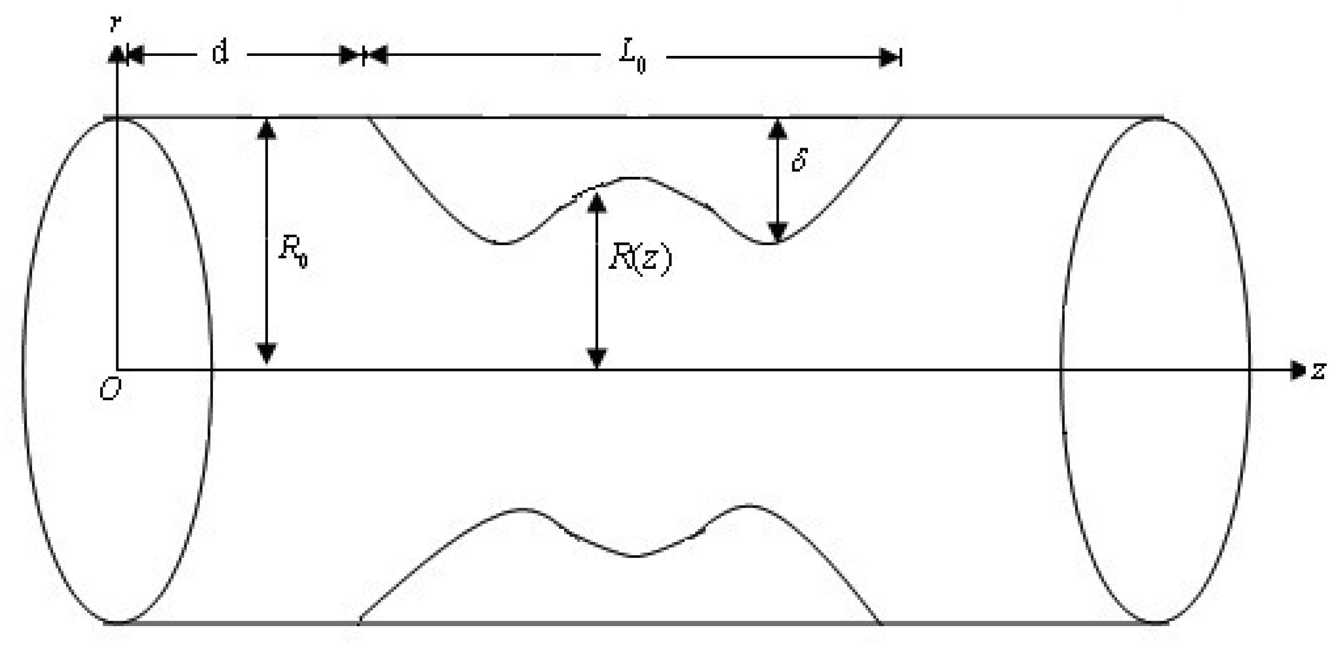
length of damaged stenotic region;

location of stenosis;

r, z:

radial and axial coordinates, respectively;

R(z):

radius of stenotic region;

R₀:

radius of non-stenotic region;

δ:

maximum radius of stenotic region;

blood velocity vector along the axial direction;

blood velocity vector along the radial direction;

solute concentration;

D₀:

diffusivity coefficient;

E₀:

reaction constant;

ρ:

density;

blood pressure;

permeability of the porous medium;

µ_s:

variable blood;

µ:

dynamic viscosity of the plasma in the blood;

λ:

maximum hematocrit at the center of cylindrical tube;

parameter used for the formula's constriction;

γ:

small parameter defined as the ratio of R₀ to L₀;

F₁:

flow resistance;

τ_w0:

wall shear stress of zeroth order;

τ_w1:

wall shear stress of 1st order

1. Introduction

Currently, the utility of robots in fulfilling various tasks in place of human beings in industrial production and daily life is gaining a significant importance. For instance, robots outperform human beings in many operations like welding, cutting, punching, paint spraying, treatment of heavy materials and sophisticated material processing ^[1]. In the grasping operations of the robots, frequent changes are associated in the poses of the target objects. To make robotic grasping more adaptive, robots have to regulate their motions on a real-time basis based on the information about object poses.

At present, more studies focus on the robotic grasping based on machine visions. Firstly, the vision-based robots need to visually determine the poses of objects. Then, coordinates of robots’ joints are determined through inverse kinetics. At last, the motions of the robots are planned by the designed motion planner. In this process, it is necessary to calibrate the visual systems. The operators need to be highly professional by traditional visual calibration methods ^[2,3,4]. Meanwhile, the computations involved in the process are very time-consuming. Besides, it is difficult to determine the inverse solutions for robots with new structures or redundant degrees of freedom. Finally, the planner design is a little complicated, which may cause other problems.

Researchers satisfied the present needs for robotic grasping by different methods; some studies were devoted to equip the end actuators with sensors such as tactile feedbacks ^[5], while some studies improved the end actuators to make robots more adaptive to grasping, for instance, D. Petković presented a novel design of an adaptive neuro fuzzy inference strategy (ANFIS) for controlling the input displacement of a new adaptive compliant gripper ^[6]. The use of embedded sensors in a robot gripper offered the control system, the ability to control the input displacement of the gripper and to recognize particular shapes of the grasping objects. Some studies focused on increasing the underactuated degree of freedom ^[7], and some studies used flexible materials ^[8] to manufacture more flexible end actuators. C. Qian et al. designed the robotic arms with 12 degrees of freedom based on multi-sensor fusion ^[9]. In these robotic arms, the sensors were used in combination with the controllers. It presented general shapes of objects through information fusion, and endowed the robotic arms with bionic functions. In consideration of the considerable costs in motor control and poor control precision of the robotic arms, S. Liu et al. designed the STM32-based robotic arms ^[10]. In this way, problems such as inaccurate motor positioning and considerable costs were effectively avoided. In addition, these robotic arms could be controlled more easily and flexibly. Although, the aforementioned methods are effective for increasing adaptivity of the robots’ end actuators, they are only useful for robots to grasp objects within the scope of work of the end actuators.

Many researchers identified the poses of objects visually and adjusted the robots’ motions for the purpose to grasp objects. Saxena et al. identified the positions and shapes of the target objects by analyzing several images of the objects, so as to draft suitable strategies for robotic grasping ^[11]. W. Dong introduced the computer visions in the original industrial transport robots ^[12]. They obtained information about the workpieces and surroundings by machine vision. Then, they identified the target workpieces to be operated and made decisions to guide the industrial robots to grasp and place workpieces.

Currently, more and more researchers have introduced the “intelligence” into grasping. They performed deep learning and training for robotic arms and gained some outcomes. Z. Yan et al. proposed a method for detecting the robots’ grasping positions based on deep learning ^[13]. In this method, the multimodal features of the target objects were employed as the training data. Robots learnt about the optimal grasping positions of target objects through unsupervised and supervised learning. In this way, they could accurately identify the optimal grasping positions of the target objects. Xia Jing put forward a rapid detection method of robot's plane grabbing posture based on cascade convolutional neural network ^[14]. He built a cascaded two-stage convolutional neural network model and used transfer learning to train models on small data sets. The results of online robotic grasping experiments showed that the method can quickly calculate the optimal grasping point and pose for irregular objects with arbitrary poses and different shapes. Its recognition accuracy and speed are improved compared with previous methods, and its robustness and stability are strong.

Robots can acquire skills for fulfilling the tasks from the people’s presentations. Y. Mollard ^[15] made a rapid and intuitive programming by demonstration of robot. K. Bousmalis ^[16] studied the effect of the randomized simulated environments and domain adaptation methods in training a grasping system to grasp novel objects from raw monocular RGB images. Asa result, they were able to reduce the number of real-world samples needed to achieve a given level of performance, by up to 50 times. Max Schwarz et al. proposed a deep object perception pipeline ^[17]. This method quickly and efficiently adapted to the new items using a custom turntable capture system and transfer learning. It produced high-quality item segments, on which grasp poses were found. Philipp Schmidt presented a data-driven, bottom-up, deep learning approach to robotic grasping of unknown objects using Deep Convolutional Neural Networks (DCNNs) ^[18]. They demonstrated the performance of our approach in qualitative grasping experiments on the humanoid robot ARMAR-III.

Earlier, we proposed a robot demonstration method based on the combination of locally weighted regression (LWR) and Q-learning algorithm ^[19]. This method adapted to the work task by learning from the demonstration and generating new actions. In literature ^[20], we built models in the Gaussian process to develop the relationship between the observable variables and the joint variables. Then the robot was able to adaptively grasp the target objects. However, adaptive grasping is only realized within relatively small training areas when models are built in a Gaussian process. If an area for object distribution is enlarged and extends to the untrained area, the effectiveness of this modelling method for robotic grasping gets greatly weakened, and the success rate of robotic grasping, in turn, gets lower.

In view of these problems, this paper proposes a robotic grasping method based on the improved Gaussian mixture models. The coordinates of the targets were extracted through a camera to get some samples for teaching. The relationships between observable variables and robots’ joint angles were mapped by the improved Gaussian models. Furthermore, the Gaussian models gained via training were used as prior models and integrated into the process of semi-supervised self-taught learning. By self-taught learning of grasping, robots grasped objects in new adjacent areas and new training samples were collected. Then we updated the probability distribution of the entire Gaussian process, obtained the posterior probabilistic models and achieved a higher success rate of grasping. For this purpose, models were built for simulation based on V-REP ^[21,22,23]. Then, they were compared with the original and improved Gaussian models in success rate of grasping. Besides, test areas where grasping by all three methods failed were analyzed in terms of positional deviation. At last, it was found that the improved Gaussian models were more adaptive.

2. Gaussian model and EM algorithms

Gaussian model precisely quantifies things using Gaussian probability density functions (normal distribution curves). It decomposes one thing into several Gaussian probability density functions (normal distribution curves).

The Expectation-Maximization (EM) algorithms are optimal algorithms for the estimation of the maximum likelihood. In general, they are used in place of the Newton’s iteration. Meanwhile they are used for estimating the parameters of the probabilistic models containing latent variables or missing data. The standard computational framework for EM algorithms is alternately composed of E and M steps. The algorithms are convergent, so they are useful for ensuring that iteration can at least approach local maximum.

Robots have to regulate themselves to adapt to objects in the process of grasping.

$f:o \to r$

(1)

In Figure 1 and Formula (1), o is an observable variable of objects, so is o_i; r is robot’s joint variable corresponding to the observable variable, so is r_i; f is mapping of the observable variable into the joint variable. Assuming that X = {x₁, x₂, …, x_n} is a set of training samples obtained through demonstration, where x_i = [r_i, o_i]^Tis a single training sample (vector) made up of joint variables and observable variables. In the process of its work, the robot firstly learn from the set of training samples (X) to get the mapping function (f); when the new observable variable (o^new) is determined, corresponding joint variable (r^new) is calculated based on the mapping function (f).

Figure 1. Observable variables and joint variables.

DownLoad: Full-Size Img PowerPoint

Selecting a suitable model to describe the mapping function (f) is fairly suitable for robots to learn about grasping. In this paper, modelling was performed by the improved Gaussian mixture models, to map the relationships between the observable variables of objects and the joint variables of robots. The models were trained with EM algorithms, and training samples were divided into several categories. Each type of samples followed a kind of Gaussian distribution and corresponded to one area.

A Gaussian mixture model was a linear superposition of several Gaussian distributions. For probability distribution of a Gaussian mixture model, the appearance probability of the sample x° is as follows:

$p({x^o}) = \sum\limits_{k = 1}^m {p(k)p({x^o}|k) = \sum\limits_{k = 1}^m {{a_k}N({x^o};{\mu _k}, {{\sum {} }_k})} }$

(2)

Where, m is total number of Gaussian distributions; p(k)-α(k) is the probability of the k^th Gaussian distribution from the sample x^o; p(x^O|k) = N(x^O; μ_k; Σ_k) is the probability of the sample x^o generated by the k^th Gaussian distribution; μ_k and ∑_k are mean vector and covariance matrix of the k^th Gaussian distribution respectively.

Samples were trained by EM algorithms of Gaussian mixture models and categorized. A work area was designated for each kind of samples. The relationships between observable variables of objects and joint variables of robots were mapped. After model parameters were initialized, E-step and M-step were iterated to constantly update model parameters until they are converged:

E-step: calculate the weight (r_ik) of the k^th Gaussian distribution from the i^th sample (x_i).

${r_{ik}} = p(k|{x_i}) = \frac{{{\alpha _k}N({x_i};{\mu _k}, {\sum _k})}}{{\sum\limits_{j = 1}^m {{\alpha _j}N({x_i};{\mu _j}, {\sum _j})} }}$

(3)

M-step: update parameters of each cluster.

${n_k} = \sum\limits_{i = 1}^n {{r_{ik}}, {\alpha _k} = \frac{{{n_k}}}{n}} \\ {\mu _k} = \sum\limits_{i = 1}^n {{r_{ik}}{x_i}} \\ \sum\nolimits_k { = \frac{{\sum\limits_{i = 1}^n {{r_{ik}}({x_i} - {\mu _k}){{({x_i} - {\mu _k})}^T}} }}{{{n_k}}}} \\$

(4)

While robots were grasping objects based on improved Gaussian model, the observable variables of the objects were identified through a camera to calculate the posterior probability of these variables in each Gaussian distribution. The robots’ joint coordinates were determined by a regression of the improved Gaussian process corresponding to the maximum posterior probability. Then robots were able to grasp the objects successfully.

3. Control methods for robotic grasping based on improved Gaussian models

3.1. Principles of robotic grasping methods based on improved Gaussian models

Principles of robotic grasping methods based on improved Gaussian models are shown in Figure 2:

Figure 2. Robotic grasping methods based on improved Gaussian models.

DownLoad: Full-Size Img PowerPoint

(1) Relationships between observable variables of target objects and corresponding robots’ joint variables were mapped using original Gaussian models. Then we identified the overall mapped relationships based on data regarding 12 groups of samples.

(2) Target positions were randomly selected in new training areas as inputs of Gaussian processes. Joint angles were predicted as the outputs. In simulation models, positive solutions were determined on the basis of joint angles. Positions of the corresponding pixel coordinates at ends of robots were observed and recorded. If the predicted and actual positions deviated by Δd less than 10 mm, the newly determined robots’ joint angles were regarded as new samples to input and update the training sets of Gaussian processes, in order to update the entire distribution process. When cumulative values reached the thresholds, it meant that enough samples were additionally obtained from the new training areas. Then posterior Gaussian distribution in the new training areas was identified.

3.2. Control Methods for Robotic Grasping Based on Improved Gaussian Models

Gaussian process modelling (GPM) method is a hypothesis for following joint normal distribution based on observable and predicted variables. We use it to calculate observable variables. Posterior probability distribution can be identified by a random input covariance matrix for training machines. GPM is a Bayesian approach, by which robots can get mapping functions from samples f. For a minority of samples, Gaussian process models can be trained. Then nonlinear connections of related variables are created.

Before data are obtained, it is assumed that joint variables and observable variables of objects follow Gaussian distribution, where the mean is μ and the covariance matrix is K:

$h: N(\mu, \mathrm{K})$

(5)

Where, h = [a, o]^T is a vector composed of observable variables and joint variables.

Meanwhile, the posterior distribution of multi-dimensional variables obtained for the sample set X is Gaussian distribution:

$p(h | X, \theta) = N\left(\mu, K+\sigma_{n}^{2} I\right)$

(6)

Where, θ = {μ, K, δ_n²} The marginal likelihood function of the sample set X is as follows:

$p = (X | H, \theta) = \prod_{(i = 1)}^{n} p\left(x_{i} | h_{i}, \theta\right) = \prod_{(i = 1)}^{n} p\left(x_{i} | h_{i}\right) p\left(h_{i} | \theta\right) = P$

(7)

Where:

$P = \prod _{\left( {i = 1} \right)}^n\frac{1}{{\sqrt {2\pi |K + \sigma _n^2I|} }}exp\left( { - \frac{{{\tau _i}}}{2}} \right)$

(8)

${\tau _i} = {\left( {{x_i} - \mu } \right)^T}{\left( {K + \sigma _n^2I} \right)^{{\rm{ - 1}}}}\left( {{x_i} - \mu } \right)$

(9)

The logarithm of the above formula is determined as follows:

$log\left( P \right) = A + B - \frac{n}{2}log\left( {2\pi } \right)$

(10)

Where:

$A = - \frac{1}{2}\sum _{\left( {i = 1} \right)}^n{\tau _i}$

(11)

$B = - \frac{n}{2}log\left| {K + \sigma _n^2I} \right|$

(12)

A and B are fitted data of the model and penalty term of model complexity respectively.

By determining partial derivatives of covariance matrix and mean vectors of the mode, the derivatives were found to be 0. The maximum likelihood estimations of the mean vectors and covariance matrix are respectively as follows:

$\mu = \frac{{\sum _{\left( {i = 1} \right)}^n{x_i}{\rm{ }}}}{n}$

(13)

$\left( {K + \sigma _n^2I} \right) = Cov({\left[ {{x_1}, {x_2}, \ldots , {x_n}} \right]^T})$

(14)

Next, it is necessary to forecast joint variables using Gaussian process models. The relationships between visual observable variables and joint variables shall be established based on teaching and training samples. At first, vectors and matrices of the Gaussian process are partitioned as follows:

$\left[ {\begin{array}{*{20}{c}} a \\ o \end{array}} \right] \sim N\left[ {\left[ {\begin{array}{*{20}{c}} {{\mu _a}} \\ {{\mu _o}} \end{array}} \right]} \right., \left. {\left[ {\begin{array}{*{20}{c}} {{K_{aa}} + \sigma _n^2I}&{{K_{ao}}} \\ {{K_{oa}}}&{{K_{oo}} + \sigma _n^2I} \end{array}} \right]} \right]$

(15)

Robots acquire information O^* about target objects through a camera, and the conditional probability distribution of corresponding joint angle a^* is as follows:

$p\left(a^{*} | o^{*}\right) = N\left(\mu_{a}^{*}, K_{a a}^{*}\right)$

(16)

Where:

$\mu _a^ * = {\mu _a} + {K_{ao}}{\left( {{K_{oo}} + \sigma _n^2I} \right)^{{\rm{ - 1}}}}\left( {{o^ * } - {\mu _o}} \right)$

(17)

$K_{aa}^ * = {K_{aa}} - {K_{ao}}{\left( {{K_{oo}} + \sigma _n^2I} \right)^{{\rm{ - 1}}}}{K_{oa}}$

(18)

μ_a^* is the mean of joint angle corresponding to the new target position. It is the maximum probability of corresponding Gaussian distribution meanwhile. The covariance matrix is K_aa^*, which reflects predictive uncertainty. If robot joint is μ_a^*, the likelihood of robotic grasping will be the highest.

By reading data of the controller, relatively accurate joint coordinates of robots are determined as follows:

$K_{aa}^ * \approx \left( {K_{aa}^ * + \sigma _n^2I} \right) = {K_{aa}} + \sigma _n^2I - {K_{ao}}{\left( {{K_{oo}} + \sigma _n^2I} \right)^{{\rm{ - 1}}}}{K_{oa}}$

(19)

In case of no visual calibration and inverse kinematic solution, target objects of the Gaussian process are closely associated with joint variables. Therefore, robots’ joint angles adaptable to target poses can be forecast according to observable variables.

The obtained Gaussian process models are deemed prior models. New models are built for the grasping in new trained areas by improved Gaussian methods. The equation is as follows:

$p(\theta | X) = \frac{p(X | \theta) \cdot p(\theta)}{p(X)}$

(20)

Where p(θ) is probability distribution of prior models; X is training sample; p(θ|X) is probability distribution of posterior models; p(X) is marginal likelihood. By the following equation, it is calculated that:

$p\left( X \right) = \smallint p\left( {X|\theta } \right)p\left( \theta \right)d\theta$

(21)

The Gaussian methods were improved for the purpose of expanding new application areas without excessively increasing sample points of original models. Therefore, this paper introduced an evaluation mechanism, in order that improved models could have expected functions after certain amount of sample points were updated. A mechanism was established for evaluating grasping in combination with the actual grasping positions. The actual positions were identified based on target positions and posterior models, so as to figure out termination requirements for posterior models. Evaluation functions were determined as follows:

$r = {S_r}{e^{{\rm{ - }}\lambda \Delta d}} + {S_r}^\prime , \Delta d = \sqrt {{{({x_a} - {x_d})}^2} + {{\left( {{y_a} - {y_d}} \right)}^2}}$

(22)

Where, S_r is the evaluated value when Δd is 0; λ is a parameter for ensuring convergence of e^-λΔd to 0 when Δd is high enough. S'_r is the value evaluated after another new sample is used.

The termination requirements for completing updates of areas are as follows:

$R = \sum _{\left( {i = 1} \right)}^n{r_i} \gt \kappa$

(23)

In other words, the new area shall be deemed to have been updated when the cumulative evaluated value reaches certain threshold.

4. Experiments

4.1. Building of the experimental platform

This robotic grasping system covered data acquisition, data processing and industrial robots, as shown in Figure 3. A UR3 robot was used. It had six spindles from the bottle to the end, including base, shoulder joint, elbow joint, wrist joint 1, wrist joint 2 and wrist joint 3. MV-EM200C/M camera was used and its resolution was 1,600*1,200. The gripper at the end was a motor-driven three-finger gripper with a single degree of freedom.

Figure 3. System components.

DownLoad: Full-Size Img PowerPoint

The experimental platform was configured as shown in Figure 4. The camera was placed above the platform. UR3 robot was on the experimental platform. The block was in the area near the black cloth. The block to be grasped was a small cube. By determining the mean of the coordinates of edge points of the block, the pixel coordinates x and y in the centre of the object were identified, as shown in Figure 5.

Figure 4. Configuration of the experimental platform.

DownLoad: Full-Size Img PowerPoint

Figure 5. Poses of the target objects.

DownLoad: Full-Size Img PowerPoint

4.2. Grasping experiment based on improved Gaussian models

The experimenter dragged the robot to the position of each block to determine the joint angles. Pixel coordinates of the blocks were obtained through a camera. Twelve experiments were performed. At last, obtained data of the observable variables and joint angles were used as training samples of models. Joint angles and pixel coordinates of the robot was recorded and utilized as training samples and input for the Gaussian process models, as shown in Table 1.

Table 1. Set of training samples.

No.	Observable Variables		Corresponding Joint Coordinates (Radian)
	Pixel (x)	Pixel (y)	Base	Shoulder Joint	Elbow Joint	Wrist Joint 1	Wrist Joint 2	Wrist Joint 3
1	239	88	-0.134	-1.730	-2.022	-0.965	1.573	0.007
2	347	88	0.003	-1.661	-2.103	-0.951	1.574	0.145
3	455	87	0.149	-1.609	-2.161	-0.944	1.575	0.291
4	455	191	0.130	-1.768	-1.976	-0.970	1.574	0.271
5	347	192	0.003	-1.810	-1.920	-0.985	1.573	0.145
6	239	192	-0.118	-1.868	-1.841	-1.008	1.572	0.023
7	239	297	-0.105	-2.004	-1.639	-1.073	1.571	0.036
8	347	297	0.003	-1.953	-1.717	-1.045	1.572	0.144
9	454	296	0.116	-1.917	-1.772	-1.026	1.573	0.257
10	401	244	0.062	-1.861	-1.852	-1.003	1.573	0.204
11	293	245	-0.055	-1.907	-1.785	-1.024	1.572	0.086
12	293	140	-0.062	-1.767	-1.977	-0.973	1.573	0.079

| Show Table

DownLoad: CSV

Table 2. New sample set.

No.	Pixel (x)	Pixel (y)	Position Error (Δd)	Base	Shoulder Joint	Elbow Joint	Wrist Joint 1	Wrist Joint 2	Wrist Joint 3
1	560	88	5.26	0.253	-1.568	-2.232	-0.912	1.576	0.395
2	668	192	1.63	0.378	-1.662	-2.107	-0.942	1.576	0.520
3	560	192	8.86	0.252	-1.713	-2.041	-0.960	1.575	0.394
4	722	244	8.64	0.440	-1.709	-2.045	-0.957	1.576	0.582
5	615	245	4.02	0.316	-1.761	-1.977	-0.975	1.575	0.458
6	614	140	7.57	0.315	-1.615	-2.170	-0.927	1.576	0.457

| Show Table

DownLoad: CSV

After training samples were obtained, the mean vector of the Gaussian process μ and the maximum likelihood estimation of covariance matrix(K+δ_n²I)were determined. The new observable variables and robot’s joint coordinates followed the same probability distribution. In case, if there was any new observable input o^*, the joint angles μ_a^* were obtained that the robot was most likely to grasp at, so as to make grasping successful.

Figure 6 shows the pixel coordinates and the corresponding joint angles of training samples. The joint angles of the base, shoulder joint, elbow joint, wrist joint 1, wrist joint 2 and wrist joint 3 were allocated from the bottom to the top. Figure 7 shows the distribution and grasping status of the training samples and the test samples on the pixel plane. The squares represent the training samples, hollow circles were successfully grasped test samples, and the solid circles were the test samples that were not successfully grasped. It is evident from the figure that the Gaussian models were helpful in the successful grasping in areas within the set of the training samples, but the grasping always failed outside the training areas. Hence, it is inferred that the Gaussian process models function fairly well within the training areas. The grasping results were not satisfactory on the boundaries near the training areas and test points outside the training areas. This suggested that the Gaussian process models were reliant upon the prior samples and were able to function well without these samples. This is a limitation of Gaussian models.

Figure 6. Joint angles of the training samples and corresponding pixel coordinates.

DownLoad: Full-Size Img PowerPoint

Figure 7. Planar distribution of pixels and grasping status of training and test samples.

DownLoad: Full-Size Img PowerPoint

Sample points of new areas were cumulatively updated by the improved Gaussian models. We selected points conforming to Δd < 10 mm as new samples for updating sample sets and calculated the evaluated values, until they reached the thresholds. This experiment suggested that only six new data were needed, and this number was far lower than the number of training samples necessary for the original Gaussian models.

Figure 8 shows distribution of the robot’s joint angles. The first row lists the joint angles of the original Gaussian model, while the second row shows the joint angles that were determined after the update of six sample points. It is evident that changes occurred to these joint angles. In particular, these changes were rather significant for the wrist joints 2 and 3, which suggested that the joint angles for grasping changed considerably in the new mapping relationships after the update.

Figure 8. Distribution of joint angles.

DownLoad: Full-Size Img PowerPoint

In order that the experiment could be accurate and generalized, this paper modelled and simulated the grasping based on VREP. As shown in Figure 9, The UR3 and blocks were put on the table and a camera was placed above them. We compared the success rate of the grasping among the original Gaussian model for grasping real objects, the improved Gaussian model for grasping simulation based on VREP and the improved Gaussian model for grasping real objects, as shown in Figures 10-12.

Figure 9. V-REP based simulation platform.

DownLoad: Full-Size Img PowerPoint

Figure 10. Success rate of grasping by the original gaussian model.

DownLoad: Full-Size Img PowerPoint

Figure 11. Success rate of VREP-based grasping simulation.

DownLoad: Full-Size Img PowerPoint

Figure 12. Success rate of grasping by the improved gaussian model.

DownLoad: Full-Size Img PowerPoint

Sixty points of the new area were randomly selected for testing, the test results are shown in Figure 10–12. The red solid circles indicted successful grasping and the hollow circles reflected failed grasping. According to the results, the success rate of direct grasping by the original Gaussian model was only 18.3%. The points for successful grasping were consisted in adjacency to the original area. The success rate of grasping by VREP-based simulations and improved Gaussian model was 81.7%, while the success rate of grasping by the improved Gaussian model was 75%. The success rate of the improved Gaussian model was slightly lower than the success rate of the simulation, possibly due to the errors in the precision of the camera sensor and robotic arm. This suggested that the improved Gaussian model could achieve more desirable grasping results in untrained areas after a minority of samples were updated.

In addition, we analysed the positional deviations for the 11 points where the grasping failed in any of the three methods. We got their positional deviation (Δd) between the statistical points and gripper end, as shown in Figure 13. It was observed that the displacement deviation was the highest in the original Gaussian model, displacement deviation of the improved Gaussian model was higher than that of V-REP simulation but far lower than that of the original Gaussian model. This indirectly suggested that the improved Gaussian model was much more adaptive than the original model even in areas where grasping failed.

Figure 13. Analysis of positional deviations in areas of failed grasping.

DownLoad: Full-Size Img PowerPoint

5. Conclusion

In this paper, a robotic grasping method based on the improved Gaussian model was put forward. This method was effective for grasping, as like the Gaussian models. It associated the observable variables with joint angles, trained areas with a minority of samples and successfully predicted the grasping at points of training areas without calibrating the visual systems. Unlike the original Gaussian model which was ineffective for predicting grasping results outside training areas, the improved model predicted grasping and achieved desirable results only by upgrading a minority of samples without any need for training samples in large areas. Finally, comparative tests were performed on real grasping, VREP-based grasping simulations by the improved Gaussian model and positional deviation analysis on areas of failed grasping. The experimental results validated the effectiveness of the method proposed in this paper.

Conflict of Interest

The authors declare there is no conflict of interest.

Acknowledgments

The authors are thankful for reviewers' comments and suggestions for an earlier version of this work that improved the quality of the present paper. S.O. thanks UTRGV for the office space and hospitality during summer of 2022 and winter of 2022.

Conflict of interest

The authors declare no conflict of interest.

Author contributions

The authors contributed equally on the completion of this manuscript.

References

[1]	Srivastava LM, Srivastava VP (1983) On two-phase model of pulsatile blood flow with entrance effects. Biorheology 20: 761-777. https://doi.org/10.3233/BIR-1983-20604
[2]	Srivastava VP, Mishra S (2010) Non-Newtonian arterial blood flow through an overlapping stenosis. Appl Appl Math 5: 225-238. https://digitalcommons.pvamu.edu/aam/vol5/iss1/17
[3]	Venkateswarlu K, Rao JA (2004) Numerical solution of unsteady blood flow through indented tube with atherosclerosis. Indian J Biochem Bio 41: 241-245.
[4]	Back LH (1994) Estimated mean flow resistance during coronary artery catheterization. J Biomech 27: 169-175. https://doi.org/10.1016/0021-9290(94)90205-4
[5]	Back LH, Kwack EY, Back MR (1996) Flow rate-pressure drop relation to coronary angioplasty: catheter obstruction effect. J Biomed Eng 118: 83-89. https://doi.org/10.1115/1.2795949
[6]	Khanduri U, Sharma BK (2022) Hall and ion slip effects on hybrid nanoparticles (Au-GO/blood) flow through a catheterized stenosed artery with thrombosis. Proc Inst Mech Eng Part C 2022: 09544062221136710. https://doi.org/10.1177/09544062221136710
[7]	Saleem A, Akhtar S, Nadeem S, et al. (2021) Microphysical analysis for peristaltic flow of SWCNT and MWCNT carbon nanotubes inside a catheterised artery having thrombus: irreversibility effects with entropy. Int J Exergy 34: 301-314. https://doi.org/10.1504/IJEX.2021.113845
[8]	Srivastava VP, Rastogi R (2010) Blood flow through a stenosed catheterized artery: Effects of hematocrit and stenosis shape. Comput Math Appl 59: 1377-1385. https://doi.org/10.1016/j.camwa.2009.12.007
[9]	Riahi DN (2016) Modeling unsteady two-phase blood flow in catheterized elastic artery with stenosis. Eng Sci Technol Int J 19: 1233-1243. https://doi.org/10.1016/j.jestch.2016.01.002
[10]	Srivastava VP (1996) Two-phase model of blood flow through stenosed tubes in the presence of a peripheral layer: applications. J Biomech 29: 1377-1382. https://doi.org/10.1016/0021-9290(96)00037-1
[11]	Back LH, Cho YI, Crawford DW, et al. (1984) Effect of mild atherosclerosis on flow resistance in a coronary artery casting of man. Trans ASME 106: 48-53. https://doi.org/10.1115/1.3138456
[12]	Riahi DN (2017) On low frequency oscillatory elastic arterial blood flow with stenosis. Int J Appl Comput Math 3: 55-70. https://doi.org/10.1007/s40819-017-0341-5
[13]	Saleem S, Akhtar S, Nadeem S, et al. (2021) Mathematical study of electroosmotically driven peristaltic flow of Casson fluid inside a tube having systematically contracting and relaxing sinusoidal heated walls. Chinese J Phys 71: 300-311. https://doi.org/10.1016/j.cjph.2021.02.015
[14]	Khaled ARA, Vafai K (2003) The role of porous media in modeling flow and heat transfer in biological tissues. Int J Heat and Mass Transfer 46: 4989-5003. https://doi.org/10.1016/S0017-9310(03)00301-6
[15]	Lee DY, Vafai K (1999) Analytical characterization and conceptual assessment of solid and fluid temperature differentials in porous media. Int J Heat and Mass Transfer 42: 423-435. https://doi.org/10.1016/S0017-9310(99)00166-0
[16]	Mann KG, Nesheim ME, Church WR, et al. (1990) Surface-dependent reactions of the vitamin K-dependence enzyme complexes. Blood 76: 1-16. https://doi.org/10.1182/blood.V76.1.1.1
[17]	Orizaga S, Riahi DN, Soto JR (2020) Drug delivery in catheterized arterial blood flow with atherosclerosis. Results Appl Math 7: 100117. https://doi.org/10.1016/j.rinam.2020.100117
[18]	Ponalagusamy R, Murugan D, Priyadharshini S (2022) Effect of rheology of non-Newtonian fluid and chemical reaction on a dispersion of a solute and implication to blood flow. Int J Appl Comput Math 8: 109. https://doi.org/10.1007/s40819-022-01312-6
[19]	Rana J, Murthy P (2017) Unsteady solute dispersion in small blood vessel using a two-phase Casson model. Proc R Soc A 473: 20170427. https://doi.org/10.1098/rspa.2017.0427
[20]	Roy AK, Bég OA (2021) Mathematical modeling of unsteady solute dispersion in two fluids (micropolar-Newtonian) blood flow with bulk reaction. Int Commun Heat Mass Transfer 122: 105169. https://doi.org/10.1016/j.icheatmasstransfer.2021.105169
[21]	Valencia A, Villanueva M (2006) Unsteady flow and mass transfer in models of stenotic arteries considering fluid-structure interaction. Int Commun Heat Mass Transfer 33: 966-975. https://doi.org/10.1016/j.icheatmasstransfer.2006.05.006
[22]	Gandhi R, Sharma BK, Kumawat C, et al. (2022) Modeling and analysis of magnetic hybrid nanoparticle (Au-Al2O3/blood) based drug delivery through a bell-shaped occluded artery with joule heating, viscous dissipation and variable viscosity effects. Proc Inst Mech Eng Part E 236: 2024-2043. https://doi.org/10.1177/09544089221080273
[23]	Khanduri U, Sharma BK (2022) Entropy analysis for mhd flow subject to temperature-dependent viscosity and thermal conductivity. Nonlinear Dynamics and Applications: Proceedings of the ICNDA 2022. Cham: Springer International Publishing 457-471. https://doi.org/10.1007/978-3-030-99792-2_38
[24]	Sharma BK, Kumawat C (2021) Impact of temperature dependent viscosity and thermal conductivity on MHD blood flow through a stretching surface with ohmic effect and chemical reaction. Nonlinear Eng 10: 255-271. https://doi.org/10.1515/nleng-2021-0020
[25]	Sharma M, Sharma B, Tripathi B (2022) Radiation effect on MHD copper suspended nanofluid flow through a stenosed artery with temperature-dependent viscosity. Int J Nonlinear Anal Appl 13: 2573-2584. http://dx.doi.org/10.22075/ijnaa.2021.22438.2362
[26]	Zhao T, Khan MR, Chu Y, et al. (2021) Entropy generation approach with heat and mass transfer in magnetohydrodynamic stagnation point flow of a tangent hyperbolic nanofluid. Appl Math Mech 42: 1205-1218. https://doi.org/10.1007/s10483-021-2759-5
[27]	Chen Z, Ma X, Zhan H, et al. (2022) Experimental investigation of solute transport across transition interface of porous media under reversible flow direction. Ecotox Environ Safe 238: 111566. https://doi.org/10.1016/j.ecoenv.2022.113566
[28]	Berkowitz B, Cortis A, Dror I, et al. (2009) Laboratory experiments on dispersive transport across interfaces: The role of flow direction. Water Resour Res 45: W02201. https://doi.org/10.1029/2008WR007342
[29]	Murugan D, Roy AK, Ponalagusamy R, et al. (2022) Tracer dispersion due to pulsatile casson fluid flow in a circular tube with chemical reaction modulated by externally applied electromagnetic fields. Int J Appl Comput Math 8: 221. https://doi.org/10.1007/s40819-022-01412-3
[30]	Ndenda JP, Shaw S, Njagarah JBH (2023) Shear induced fractionalized dispersion during Magnetic Drug Targeting in a permeable microvessel. Colloids Surf B 221: 113001. https://doi.org/10.1016/j.colsurfb.2022.113001
[31]	Roy AK, Bég OA (2021) Asymptotic study of unsteady mass transfer through a rigid artery with multiple irregular stenoses. Appl Math Comput 410: 126485. https://doi.org/10.1016/j.amc.2021.126485
[32]	Roy AK, Saha AK, Ponalagusamy R, et al. (2020) Mathematical model on magneto-hydrodynamic dispersion in a porous medium under the influence of bulk chemical reaction. Korea-Aust Rheol J 32: 287-299. https://doi.org/10.1007/s13367-020-0027-0
[33]	Sharma MK, Bansal K, Bansal S (2012) Pulsatile unsteady flow of blood through porous medium in a stenotic artery under the influence of transverse magnetic field. Korea-Aust Rheol J 24: 181-189. https://doi.org/10.1007/s13367-012-0022-1
[34]	Lapwood ER (1948) Convection of a fluid in a porous medium. Proceedings of the Cambridge Philosophical Society. UK: Cambridge University Press 508-521. https://doi.org/10.1017/S030500410002452X
[35]	White FM (1991) Viscous Fluid Flow. New York: McGraw-Hill Inc.
[36]	Sinha A, Shit GC (2015) Modeling of blood flow in a constricted porous vessel under magnetic environment: an analytical approach. Int J App Comput Math 1: 219-234. https://doi.org/10.1007/s40819-014-0022-6
[37]	Ascher U, Mathheij RM, Russell RD (1995) Numerical Solution of Boundary Value Problems for Ordinary Differential Equations. Philadelphia: SIAM Publication. https://doi.org/10.1137/1.9781611971231

This article has been cited by:

1.	Mingjun Ye , Heng Zhou, Haoyu Yang, Bin Hu, Xiong Wang, Multi-Strategy Improved Dung Beetle Optimization Algorithm and Its Applications, 2024, 9, 2313-7673, 291, 10.3390/biomimetics9050291
2.	Xiong Wang, Yaxin Wei, Zihao Guo, Jihong Wang, Hui Yu, Bin Hu, A Sinh–Cosh-Enhanced DBO Algorithm Applied to Global Optimization Problems, 2024, 9, 2313-7673, 271, 10.3390/biomimetics9050271
3.	Shuwan Feng, Jihong Wang, Ziming Li, Sai Wang, Ziyi Cheng, Hui Yu, Jiasheng Zhong, Research on Move-to-Escape Enhanced Dung Beetle Optimization and Its Applications, 2024, 9, 2313-7673, 517, 10.3390/biomimetics9090517
4.	Shihua Li, Yanjie Zhou, Bing Zhou, Zongmin Wang, Workload-based adaptive decision-making for edge server layout with deep reinforcement learning, 2025, 139, 09521976, 109662, 10.1016/j.engappai.2024.109662

Reader Comments

Your name:*

Email:*
© 2023 the Author(s), licensee AIMS Press. This is an open access article distributed under the terms of the Creative Commons Attribution License (http://creativecommons.org/licenses/by/4.0)