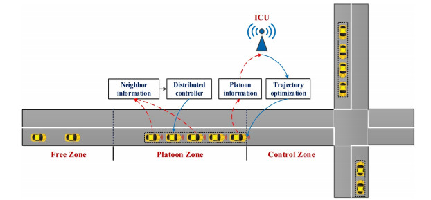
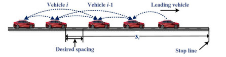
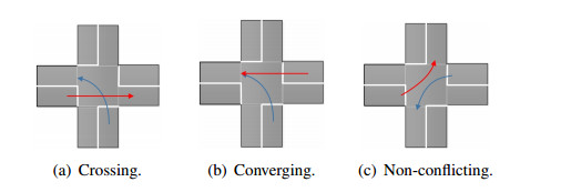
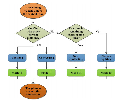
This paper proposes a distributed collision-free control scheme for connected and automated vehicles (CAVs) at a non-signalized intersection. We first divide an intersection area into three sections, i.e., the free zone, the platoon zone, and the control zone. In order to enable the following vehicles to track the trajectory of their leading vehicle in the platoon zone and the control zone, as well as to guarantee the desired distance between any two adjacent vehicles, the distributed platoon controllers are designed. In the control zone, each vehicular platoon is taken as a whole to be coordinated via an intersection coordination unit (ICU). To avoid collision between each pair of the conflicting platoons approaching from different directions, a platoon-based coordination strategy is designed by scheduling the arrival time of each leading vehicle of different platoons. Specially, considering traffic efficiency and fuel economy, the optimal control problem of the leading vehicle is formulated subject to the constraint of allowable minimum arrival time, which is derived from coordination with other approaching platoons. The Pontryagin Minimum Principle (PMP) and phase-plane method are applied to find the optimal control sequences. Numerical simulations show the effectiveness of this scheme.
Citation: Jian Gong, Yuan Zhao, Jinde Cao, Wei Huang. Platoon-based collision-free control for connected and automated vehicles at non-signalized intersections[J]. Electronic Research Archive, 2023, 31(4): 2149-2174. doi: 10.3934/era.2023111
This paper proposes a distributed collision-free control scheme for connected and automated vehicles (CAVs) at a non-signalized intersection. We first divide an intersection area into three sections, i.e., the free zone, the platoon zone, and the control zone. In order to enable the following vehicles to track the trajectory of their leading vehicle in the platoon zone and the control zone, as well as to guarantee the desired distance between any two adjacent vehicles, the distributed platoon controllers are designed. In the control zone, each vehicular platoon is taken as a whole to be coordinated via an intersection coordination unit (ICU). To avoid collision between each pair of the conflicting platoons approaching from different directions, a platoon-based coordination strategy is designed by scheduling the arrival time of each leading vehicle of different platoons. Specially, considering traffic efficiency and fuel economy, the optimal control problem of the leading vehicle is formulated subject to the constraint of allowable minimum arrival time, which is derived from coordination with other approaching platoons. The Pontryagin Minimum Principle (PMP) and phase-plane method are applied to find the optimal control sequences. Numerical simulations show the effectiveness of this scheme.

| [1] | B. Jeremy, T. Pete, K. Alan, B. Laurie, Y. George, E. Petros, et al., Traffic safety basic facts 2012: junctions, 2013. Available from: https://roderic.uv.es/handle/10550/30218. |
| [2] | NHTSA, Fatality Analysis Reporting System (FARS). Available from: http://www.nhtsa.gov/FARS. |
| [3] | P. B. Hunt, D. I. Robertson, R. D. Bretherton, R. I. Winton, SCOOT-a traffic responsive method of coordinating signals, 1981. Available from: https://trid.trb.org/view/179439. |
| [4] |
A. G. Sims, K. W. Dobinson, The Sydney coordinated adaptive traffic (SCAT) system philosophy and benefits, IEEE Trans. Veh. Technol., 29 (1980), 130–137. https://doi.org/10.1109/T-VT.1980.23833 doi: 10.1109/T-VT.1980.23833

|
| [5] |
S. C. Wong, W. T. Wong, C. M. Leung, C. O. Tong, Group-based optimization of a time-dependent TRANSYT traffic model for area traffic control, Abbreviation Title Transp. Res. Part B Methodol., 36 (2002), 291–312. https://doi.org/10.1016/S0191-2615(01)00004-2 doi: 10.1016/S0191-2615(01)00004-2
|
| [6] |
L. Chen, C. Englund, Cooperative intersection management: a survey, IEEE Trans. Intell. Transp. Syst., 17 (2015), 570–586. https://doi.org/10.1109/TITS.2015.2471812 doi: 10.1109/TITS.2015.2471812
|
| [7] |
S. El-Tantawy, B. Abdulhai, H. Abdelgawad, Multiagent reinforcement learning for integrated network of adaptive traffic signal controllers (MARLIN-ATSC): methodology and large-scale application on downtown Toronto, IEEE Trans. Intell. Transp. Syst., 14 (2013), 1140–1150. https://doi.org/10.1109/TITS.2013.2255286 doi: 10.1109/TITS.2013.2255286
|
| [8] |
A. Zaidi, B. Kulcsár, H. Wymeersch, Back-pressure traffic signal control with fixed and adaptive routing for urban vehicular networks, IEEE Trans. Intell. Transp. Syst., 17 (2016), 2134–2143. https://doi.org/10.1109/TITS.2016.2521424 doi: 10.1109/TITS.2016.2521424
|
| [9] | K. Dresner, P. Stone, Multiagent traffic management: a reservation-based intersection control mechanism, in Proceedings of the Third International Joint Conference on Autonomous Agents and Multiagent Systems, (2005), 471–477. https://doi.org/10.1145/1082473.1082545 |
| [10] |
K. Dresner, P. Stone, A multiagent approach to autonomous intersection management, J. Artif. Intell. Res., 31 (2008), 591–656. https://doi.org/10.1613/jair.2502 doi: 10.1613/jair.2502
|
| [11] |
M. Ahmane, A. Abbas-Turki, F. Perronnet, J. Wu, A. E. Moudni, J. Buisson, et al., Modeling and controlling an isolated urban intersection based on cooperative vehicles, Transp. Res. Part C Emerging Technol., 28 (2013), 44–62. https://doi.org/10.1016/j.trc.2012.11.004 doi: 10.1016/j.trc.2012.11.004
|
| [12] |
L. Li, F. Wang, Cooperative driving at blind crossings using intervehicle communication, IEEE Trans. Veh. Technol., 55 (2006), 1712–1724. https://doi.org/10.1109/TVT.2006.878730 doi: 10.1109/TVT.2006.878730
|
| [13] |
J. Lee, B. Park, Development and evaluation of a cooperative vehicle intersection control algorithm under the connected vehicles environment, IEEE Trans. Intell. Transp. Syst., 13 (2012), 81–90. https://doi.org/10.1109/TITS.2011.2178836 doi: 10.1109/TITS.2011.2178836
|
| [14] |
M. A. S. Kamal, J. Imura, T. Hayakawa, A. Ohata, K. Aihara, A vehicle-intersection coordination scheme for smooth flows of traffic without using traffic lights, IEEE Trans. Intell. Transp. Syst., 16 (2014), 1136–1147. https://doi.org/10.1109/TITS.2014.2354380 doi: 10.1109/TITS.2014.2354380
|
| [15] |
P. Dai, K. Liu, Q. Zhuge, E. H. Sha, V. C. S. Lee, S. H. Son, Quality-of-experience-oriented autonomous intersection control in vehicular networks, IEEE Trans. Intell. Transp. Syst., 17 (2016), 1956–1967. https://doi.org/10.1109/TITS.2016.2514271 doi: 10.1109/TITS.2016.2514271
|
| [16] | S. E. Li, Y. Zheng, K. Li, J. Wang, An overview of vehicular platoon control under the four-component framework, in 2015 IEEE Intelligent Vehicles Symposium (IV), (2015), 286–291. https://doi.org/10.1109/IVS.2015.7225700 |
| [17] |
L. Xiao, F. Gao, Practical string stability of platoon of adaptive cruise control vehicles, IEEE Trans. Intell. Transp. Syst., 12 (2011), 1184–1194. https://doi.org/10.1109/TITS.2011.2143407 doi: 10.1109/TITS.2011.2143407
|
| [18] |
S. Darbha, S. Konduri, P. Pagilla, Benefits of V2V communication for autonomous and connected vehicles, IEEE Trans. Intell. Transp. Syst., 20 (2018), 1954–1963. https://doi.org/10.1109/TITS.2018.2859765 doi: 10.1109/TITS.2018.2859765
|
| [19] |
Y. Zheng, S. E. Li, J. Wang, D. Cao, K. Li, Stability and scalability of homogeneous vehicular platoon: study on the influence of information flow topologies, IEEE Trans. Intell. Transp. Syst., 17 (2015), 14–26. https://doi.org/10.1109/TITS.2015.2402153 doi: 10.1109/TITS.2015.2402153
|
| [20] |
S. E. Li, Y. Zheng, K. Li, Y. Wu, J. K. Hedrick, F. Gao, et al., Dynamical modeling and distributed control of connected and automated vehicles: challenges and opportunities, IEEE Intell. Transp. Syst. Mag., 9 (2017), 46–58. https://doi.org/10.1109/MITS.2017.2709781 doi: 10.1109/MITS.2017.2709781
|
| [21] |
M. Bernardo, P. Falcone, A. Salvi, S. Santini, Design, analysis, and experimental validation of a distributed protocol for platooning in the presence of time-varying heterogeneous delays, IEEE Trans. Control Syst. Technol., 24 (2015), 413–427. https://doi.org/10.1109/TCST.2015.2437336 doi: 10.1109/TCST.2015.2437336
|
| [22] |
S. Stüdli, M. Seron, R. H. Middleton, Vehicular platoons in cyclic interconnections, Automatica, 94 (2018), 283–293. https://doi.org/10.1016/j.automatica.2018.04.033 doi: 10.1016/j.automatica.2018.04.033
|
| [23] |
F. Gao, X. Hu, S. E. Li, K. Li, Q. Sun, Distributed adaptive sliding mode control of vehicular platoon with uncertain interaction topology, IEEE Trans. Ind. Electron., 65 (2018), 6352–6361. https://doi.org/10.1109/TIE.2017.2787574 doi: 10.1109/TIE.2017.2787574
|
| [24] |
F. Gao, S. E. Li, Y. Zheng, D. Kum, Robust control of heterogeneous vehicular platoon with uncertain dynamics and communication delay, IET Intell. Transp. Syst., 10 (2016), 503–513. https://doi.org/10.1049/iet-its.2015.0205 doi: 10.1049/iet-its.2015.0205
|
| [25] |
P. Liu, A. Kurt, U. Ozguner, Distributed model predictive control for cooperative and flexible vehicle platooning, IEEE Trans. Control Syst. Technol., 27 (2018), 1115–1128. https://doi.org/10.1109/TCST.2018.2808911 doi: 10.1109/TCST.2018.2808911
|
| [26] |
A. I. M. Medina, N. V. D. Wouw, H. Nijmeijer, Cooperative intersection control based on virtual platooning, IEEE Trans. Intell. Transp. Syst., 19 (2017), 1727–1740. https://doi.org/10.1109/TITS.2017.2735628 doi: 10.1109/TITS.2017.2735628
|
| [27] |
B. Xu, S. E. Li, Y. Bian, S. Li, X. J. Ban, J. Wang, et al., Distributed conflict-free cooperation for multiple connected vehicles at unsignalized intersections, Transp. Res. Part C Emerging Technol., 93 (2018), 322–334. https://doi.org/10.1016/j.trc.2018.06.004 doi: 10.1016/j.trc.2018.06.004
|
| [28] |
Y. Zhou, M. E. Cholette, A. Bhaskar, E. Chung, Optimal vehicle trajectory planning with control constraints and recursive implementation for automated on-ramp merging, IEEE Trans. Intell. Transp. Syst., 20 (2018), 3409–3420. https://doi.org/10.1109/TITS.2018.2874234 doi: 10.1109/TITS.2018.2874234
|
| [29] |
I. Flugge-Lotz, H. Marbach, The optimal control of some attitude control systems for different performance criteria, J. Fluids Eng., 85 (1963), 165–175. https://doi.org/10.1115/1.3656552 doi: 10.1115/1.3656552
|
| [30] |
P. Wang, Y. Jiang, L. Xiao, Y. Zhao, Y. Li, A joint control model for connected vehicle platoon and arterial signal coordination, J. Intell. Transp. Syst., 24 (2020), 81–92. https://doi.org/10.1080/15472450.2019.1579093 doi: 10.1080/15472450.2019.1579093
|
| [31] |
J. Gong, J. Cao, Y. Zhao, Y. Wei, J. Guo, W. Huang, Sampling-based cooperative adaptive cruise control subject to communication delays and actuator lags, Math. Comput. Simul., 171 (2020), 13–25. https://doi.org/10.1016/j.matcom.2019.10.012 doi: 10.1016/j.matcom.2019.10.012
|
| [32] |
Y. Zhao, G. Guo, Distributed tracking control of mobile sensor networks with intermittent communications, J. Franklin Inst., 354 (2017), 3634–3647. https://doi.org/10.1016/j.jfranklin.2017.03.003 doi: 10.1016/j.jfranklin.2017.03.003
|
| [33] |
M. A. S. Kamal, M. Mukai, J. Murata, T. Kawabe, Ecological vehicle control on roads with up-down slopes, IEEE Trans. Intell. Transp. Syst., 12 (2011), 783–794. https://doi.org/10.1109/TITS.2011.2112648 doi: 10.1109/TITS.2011.2112648
|
| [34] |
B. Paden, S. Sastry, A calculus for computing Filippov's differential inclusion with application to the variable structure control of robot manipulators, IEEE Trans. Circuits Syst., 34 (1987), 73–82. https://doi.org/10.1109/TCS.1987.1086038 doi: 10.1109/TCS.1987.1086038
|
| [35] |
S. Li, X. Qin, Y. Zheng, J. Wang, K. Li, H. Zhang, Distributed platoon control under topologies with complex eigenvalues: stability analysis and controller synthesis, IEEE Trans. Control Syst. Technol., 27 (2017), 206–220. https://doi.org/10.1109/TCST.2017.2768041 doi: 10.1109/TCST.2017.2768041
|
Figures(13) / Tables(3)
Jian Gong, Yuan Zhao, Jinde Cao, Wei Huang. Platoon-based collision-free control for connected and automated vehicles at non-signalized intersections[J]. Electronic Research Archive, 2023, 31(4): 2149-2174. doi: 10.3934/era.2023111


 DownLoad: