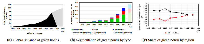
Recent years have been characterized by considerable growth of the green bond market in Europe, particularly in the domain of social bond issuance. Considering the recent pandemic, it is also a stylized fact that this growth is positively correlated with the concept of health-related uncertainty, as the green bond market aims to acquire financing in order to allow the development of projects that comply with the so-called environmental (E), social (S) and governance (G) criteria. This study then applies a dynamic spatial econometric analysis and several robustness checks to assess the extent to which each E, S and G criterion contributes to the societal dynamics of health-related uncertainty. The analysis takes advantage of available data on the number of confirmed cases of COVID-19 to measure health-related uncertainty at the municipal level, so that a higher (lower) number of confirmed cases constitutes a proxy for a greater (smaller) degree of uncertainty, respectively. To reinforce the need to evaluate impacts in a context characterized by health-related uncertainty, the time span covers the first wave of COVID-19, which is the period when uncertainty reached its highest peak. Additionally, the geographical scope is mainland Portugal since this country has become a breeding ground for startups and new ideas, being currently one of the world leaders in hosting businesses that reached Unicorn status. The main result of this research is that only the social dimension has a significant, positive and permanent impact on health-related uncertainty. Therefore, this study empirically confirms that the European green bond market has been and can be further leveraged by the need to finance projects with a social scope.
Citation: Vitor Miguel Ribeiro. Green bond market boom: did environmental, social and governance criteria play a role in reducing health-related uncertainty?[J]. Green Finance, 2023, 5(1): 18-67. doi: 10.3934/GF.2023002
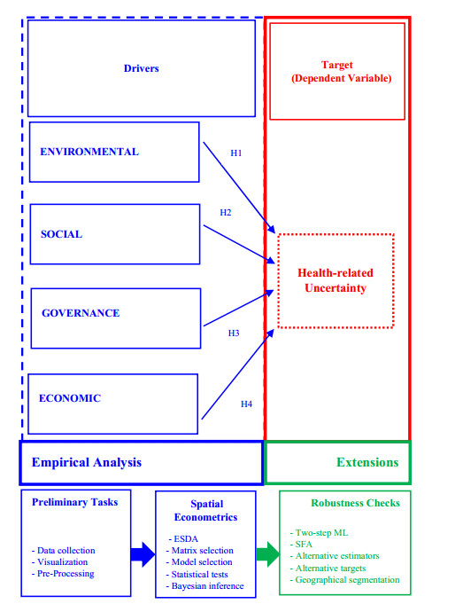
Recent years have been characterized by considerable growth of the green bond market in Europe, particularly in the domain of social bond issuance. Considering the recent pandemic, it is also a stylized fact that this growth is positively correlated with the concept of health-related uncertainty, as the green bond market aims to acquire financing in order to allow the development of projects that comply with the so-called environmental (E), social (S) and governance (G) criteria. This study then applies a dynamic spatial econometric analysis and several robustness checks to assess the extent to which each E, S and G criterion contributes to the societal dynamics of health-related uncertainty. The analysis takes advantage of available data on the number of confirmed cases of COVID-19 to measure health-related uncertainty at the municipal level, so that a higher (lower) number of confirmed cases constitutes a proxy for a greater (smaller) degree of uncertainty, respectively. To reinforce the need to evaluate impacts in a context characterized by health-related uncertainty, the time span covers the first wave of COVID-19, which is the period when uncertainty reached its highest peak. Additionally, the geographical scope is mainland Portugal since this country has become a breeding ground for startups and new ideas, being currently one of the world leaders in hosting businesses that reached Unicorn status. The main result of this research is that only the social dimension has a significant, positive and permanent impact on health-related uncertainty. Therefore, this study empirically confirms that the European green bond market has been and can be further leveraged by the need to finance projects with a social scope.

| [1] |
Adda J (2016) Economic activity and the spread of viral diseases: Evidence from high frequency data. Quart J Econ 131: 891–941. https://doi.org/10.1093/qje/qjw005 doi: 10.1093/qje/qjw005

|
| [2] |
Agliardi E, Agliardi R (2019) Financing environmentally-sustainable projects with green bonds. Environ Develop Econ 24: 608–623. https://doi.org/10.1017/S1355770X19000020 doi: 10.1017/S1355770X19000020
|
| [3] |
Aleksandrova-Zlatanska S, Kalcheva DZ (2019) Alternatives for financing of municipal investments — green bonds. Rev Econ Bus Stud 12: 59–78. https://doi.org/10.1515/rebs-2019-0082 doi: 10.1515/rebs-2019-0082
|
| [4] | Anselin L (1988) Spatial econometrics: Methods and models. Kluwer Academic: Boston, MA. ISBN: 90-247-3735-4 |
| [5] | Anselin L, Syabri I, Kho Y (2010) GeoDa: an introduction to spatial data analysis, Hand Appl Spat Anal, Springer: 73–89. https://doi.org/10.1007/978-3-642-03647-7_5 |
| [6] | APR (1986) Artigo 9 da Lei no. 44/86 da Série I do Diário da República no. 225/1986 de 1986-09-30, 2779-2783. Available from: https://dre.pt/application/conteudo/221696. |
| [7] | Barnes SR, Beland LP, Huh J, et al (2020) The Effect of COVID-19 Lockdown on Mobility and Traffic Accidents: Evidence from Louisiana. GLO Discussion Paper. Available from: https://econpapers.repec.org/paper/zbwglodps/616.htm. |
| [8] |
Barmby T, Larguem M (2009) Coughs and sneezes spread diseases: An empirical study of absenteeism and infectious illness. J Health Econ 28: 1012–1017.https://doi.org/10.1016/j.jhealeco.2009.06.006 doi: 10.1016/j.jhealeco.2009.06.006
|
| [9] |
Battese GE, Coelli TJ (1992) Frontier production functions, technical efficiency and panel data: with application to paddy farmers in India. J Prod Analy 3: 153–169. https://doi.org/10.1007/BF00158774 doi: 10.1007/BF00158774
|
| [10] |
Battese GE, Coelli TJ (1995) A model for technical inefficiency effects in a stochastic frontier production function for panel data. Empirical Econ 20: 325–332. https://doi.org/10.1007/BF01205442 doi: 10.1007/BF01205442
|
| [11] |
Bell A, Jones K (2015) Explaining fixed effects: Random effects modeling of time-series cross-sectional and panel data. Pol Sci Res Meth 3: 133–153. https://doi.org/10.1017/psrm.2014.7 doi: 10.1017/psrm.2014.7
|
| [12] | Bilgin NM (2020) Tracking COVID-19 Spread in Italy with Mobility Data. SSRN 3585921. Available from: https://econpapers.repec.org/paper/kocwpaper/2012.htm |
| [13] |
Boshcma R (2005) Proximity and innovation: a critical assessment. Reg Stud 39: 61–74. https://doi.org/10.1080/0034340052000320887 doi: 10.1080/0034340052000320887
|
| [14] |
Bhutta US, Tariq A, Farrukh M, et al (2022) Green bonds for sustainable development: Review of literature on development and impact of green bonds. Tech For Soc Change 175: 121378. https://doi.org/10.1016/j.techfore.2021.121378 doi: 10.1016/j.techfore.2021.121378
|
| [15] |
Camagni R (2017) Regional competitiveness: towards a concept of territorial capital. Sem Stud Reg Urb Econ 1: 115–131. https://doi.org/10.1007/978-3-319-57807-1_6 doi: 10.1007/978-3-319-57807-1_6
|
| [16] |
Capello R, Faggian A (2005) Collective learning and relational capital in local innovation processes. Reg Stud 39: 75–87. https://doi.org/10.1080/0034340052000320851 doi: 10.1080/0034340052000320851
|
| [17] | Caselli M, Fracasso A, Scicchitano S (2020) From the lockdown to the new normal: An analysis of the limitations to individual mobility in Italy following the Covid-19 crisis. GLO Discussion Paper. Available from: https://www.econstor.eu/handle/10419/225064 |
| [18] | CBI (2022) H1 Market Report: Green and other labelled bond volumes reach $ \$ $417.8bn in first half of 2022. Available from: https://www.climatebonds.net/resources/press-releases/2022/08/h1-market-report-green-and-other-labelled-bond-volumes-reach-4178bn |
| [19] |
Choi BB, Lee D, Park Y (2013) Corporate social responsibility, corporate governance and earnings quality: Evidence from Korea. Corp Gov: Intern Rev 21: 447-–467. https://doi.org/10.1111/corg.12033 doi: 10.1111/corg.12033
|
| [20] |
Cicchiello AF, Cotugno M, Monferrà S, et al (2022) Which are the factors influencing green bonds issuance? Evidence from the European bonds market. Fin Res Let 50: 103190. https://doi.org/10.1016/j.frl.2022.103190 doi: 10.1016/j.frl.2022.103190
|
| [21] |
Coles JL, Daniel ND, Naveen L (2008) Boards: Does one size fit all? J Fin Econ 87: 329–356. https://doi.org/10.1016/j.jfineco.2006.08.008 doi: 10.1016/j.jfineco.2006.08.008
|
| [22] |
Cornwell C, Schmidt P, Sickles RC (1990) Production frontiers with cross-sectional and time-series variation in efficiency levels. J Econometrics 46: 185–200. https://doi.org/10.1016/0304-4076(90)90054-W doi: 10.1016/0304-4076(90)90054-W
|
| [23] |
Crowley F, Doran J (2020) Covid-19, Occupational Social Distancing and Remote Working Potential: An Occupation, Sector and Regional Perspective. Reg Sci Pol Pract: 1211–1234. https://doi.org/10.1111/rsp3.12347 doi: 10.1111/rsp3.12347
|
| [24] |
Dan A, Tiron-Tudor A (2021) The determinants of green bond issuance in the European Union. J Risk Fin Manag 14: 446. https://doi.org/10.3390/jrfm14090446 doi: 10.3390/jrfm14090446
|
| [25] | Davidson R, MacKinnon JG (1993) Estimation and inference in econometrics 63. New York: Oxford University Press. https://doi.org/10.1017/S0266466600009452 |
| [26] | Deboeck GJ (1994) Trading on the edge: neural, genetic, and fuzzy systems for chaotic financial markets. London: John Wiley and Sons. ISBN: 0-471-31100-6 |
| [27] | Dell'Atti S, Tommaso C, Pacelli V (2022) Sovereign green bond and country value and risk: Evidence from European Union countries. J Intern Fin Manag Account: In press. https://doi.org/10.1111/jifm.12155 |
| [28] | EC (2022) European green bonds A standard for Europe, open to the world. Available from: https://www.europarl.europa.eu/RegData/etudes/BRIE/2022/698870/EPRS_BRI(2022)698870_EN.pdf |
| [29] | ECDPC (2018) European Center for Disease Prevention and Control Technical document - 2018 HEPSA (Health emergency preparedness self-assessment tool user guide). Stockholm: ECDC. Available from: https://www.ecdc.europa.eu/en/publications-data/hepsa-health-emergency-preparedness-self-assessment-tool-user-guide |
| [30] | Elhorst JP (2017) Spatial Panel Data Analysis. Ency GIS 2: 2050–2058. Available fom: https://spatial-panels.com/wp-content/uploads/2017/07/Elhorst-Spatial-Panel-Data-Analysis-Encyclopedia-GIS-2nd-ed_Working-Paper-Version.pdf |
| [31] | Engle S, Stromme J, Zhou A (2020) Staying at home: mobility effects of covid-19. Mimeo. Available from: https://papers.ssrn.com/sol3/papers.cfm?abstract_id=3565703 |
| [32] |
Fang H, Wang L, Yang Y (2020) Human mobility restrictions and the spread of the novel coronavirus (2019-ncov) in China. J Public Econ 191: 104272. https://doi.org/10.1016/j.jpubeco.2020.104272 doi: 10.1016/j.jpubeco.2020.104272
|
| [33] |
Fatica S, Panzica R, Rancan M (2021) The pricing of green bonds: are financial institutions special?. J Fin Stab 54: 100873. https://doi.org/10.1016/j.jfs.2021.100873 doi: 10.1016/j.jfs.2021.100873
|
| [34] | Favero CA, Ichino A, Rustichini A (2020) Restarting the economy while saving lives under Covid-19. CEPR Discussion Paper No. DP14664. Available from: https://econpapers.repec.org/paper/cprceprdp/14664.htm |
| [35] |
Firmino D, Elhorst JP, Neto RMS (2017) Urban and rural population growth in a spatial panel of municipalities. Reg Stud 51: 894–908. https://doi.org/10.1080/00343404.2016.1144922 doi: 10.1080/00343404.2016.1144922
|
| [36] |
Flammer C (2021) Corporate green bonds. J Fin Econ 142: 499–516. https://doi.org/10.1016/j.jfineco.2021.01.010 doi: 10.1016/j.jfineco.2021.01.010
|
| [37] |
Fritsch M, Kublina S (2018) Related variety, unrelated variety and regional growth: the role of absorptive capacity and entrepreneurship. Reg Stud 52: 1360–1371. https://doi.org/10.1080/00343404.2017.1388914 doi: 10.1080/00343404.2017.1388914
|
| [38] |
Gianfrate G, Peri M (2019) The green advantage: Exploring the convenience of issuing green bonds. J Clean Prod 219: 127–135. https://doi.org/10.1016/j.jclepro.2019.02.022 doi: 10.1016/j.jclepro.2019.02.022
|
| [39] | Glaeser EL, Gorback CS, Redding SJ (2020) How much does covid-19 increase with mobility? evidence from new york and four other us cities. National Bureau of Economic Research. Available from: https://www.nber.org/system/files/working_papers/w27519/w27519.pdf |
| [40] | Godzinski A, Suarez-Castillo M (2019) Short-term health effects of public transport disruptions: air pollution and viral spread channels. Mimeo. Available from: https://econpapers.repec.org/paper/nsedoctra/g2019-03.htm |
| [41] |
Greene W (2005) Fixed and random effects in stochastic frontier models. J Prod Analy 23: 7–32. doi: https://doi.org/10.1007/s11123-004-8545-1 doi: 10.1007/s11123-004-8545-1
|
| [42] |
Gilchrist D, Yu J, Zhong R (2021) The limits of green finance: A survey of literature in the context of green bonds and green loans. Sustainability 13: 478. https://doi.org/10.3390/su13020478 doi: 10.3390/su13020478
|
| [43] |
Hamilton JD, Waggoner DF, Zha T (2007) Normalization in econometrics. Econometric Rev 26: 221–252. https://doi.org/10.1080/07474930701220329 doi: 10.1080/07474930701220329
|
| [44] |
Hamilton JG, Genoff MC, Han PK (2020) Health‐Related Uncertainty. Wiley Ency Health Psych 305–313. https://doi.org/10.1002/9781119057840.ch80 doi: 10.1002/9781119057840.ch80
|
| [45] |
Han Y, Li J (2022) Should investors include green bonds in their portfolios? Evidence for the USA and Europe. Intern Rev Fin Analy 80: 101998. https://doi.org/10.1016/j.irfa.2021.101998 doi: 10.1016/j.irfa.2021.101998
|
| [46] |
Han PKJ, Klein WMP, Arora NK (2011) Varieties of uncertainty in health care: A conceptual taxonomy. Med Decis Making 31: 828–838. https://doi.org/10.1177/0272989X103939 doi: 10.1177/0272989X103939
|
| [47] |
Hancock AA, Bush EN, Stanisic D, et al (1988) Data normalization before statistical analysis: keeping the horse before the cart. Trend Pharma Sci 9: 29–32. https://doi.org/10.1016/0165-6147(88)90239-8 doi: 10.1016/0165-6147(88)90239-8
|
| [48] |
Hachenberg B, Schiereck D (2018) Are green bonds priced differently from conventional bonds?. J Asset Manag 19: 371–383. https://doi.org/10.1057/s41260-018-0088-5 doi: 10.1057/s41260-018-0088-5
|
| [49] |
Hsiang S, Allen D, Annan-Phan S, et al (2020) The effect of large-scale anti-contagion policies on the COVID-19 pandemic. Nature 584: 262–267. https://doi.org/10.1038/s41586-020-2404-8 doi: 10.1038/s41586-020-2404-8
|
| [50] |
Iacobucci G (2020) Covid-19: Deprived areas have the highest death rates in England and Wales. British Med J 369: 1. https://doi.org/10.1136/bmj.m1810 doi: 10.1136/bmj.m1810
|
| [51] |
Laborda J, Sánchez-Guerra A (2021) Green bond finance in Europe and the stock market reaction. Estud Economía Aplicada 39: 5. https://doi.org/10.25115/eea.v39i3.4125 doi: 10.25115/eea.v39i3.4125
|
| [52] | Lee YH, Schmidt P (1993). A production frontier model with flexible temporal variation in technical efficiency. The measurement of productive efficiency: Techniques and applications. 237–255. ISBN: 0-19-507218-9 |
| [53] |
Lee LF (2004) Asymptotic distributions of quasi-maximum likelihood estimators for spatial autoregressive models. Econometrica 72: 1899–1925. https://doi.org/10.1111/j.1468-0262.2004.00558.x doi: 10.1111/j.1468-0262.2004.00558.x
|
| [54] |
Lee LF, Yu J (2016). Identification of spatial Durbin panel models. J Appl Econometrics 31: 133–162. https://doi.org/10.1002/jae.2450 doi: 10.1002/jae.2450
|
| [55] |
Lee DL, McCrary J, Moreira MJ, et al (2020) Valid t-ratio Inference for Ⅳ. Amer Econ Rev 112: 3260–3290. https://doi.org/10.1257/aer.20211063 doi: 10.1257/aer.20211063
|
| [56] |
Leitao J, Ferreira J, Santibanez‐Gonzalez E (2021) Green bonds, sustainable development and environmental policy in the European Union carbon market. Bus Strat Environ 30: 2077–2090. https://doi.org/10.1002/bse.2733 doi: 10.1002/bse.2733
|
| [57] | LeSage JP, Pace RK (2009) Introduction to Spatial Econometrics. Boca Raton, FL: CRC Press. https://doi.org/10.1201/9781420064254 |
| [58] |
LeSage JP (2014) Spatial econometric panel data model specification: A Bayesian approach. Spat Stat 9: 122–145. https://doi.org/10.1016/j.spasta.2014.02.002 doi: 10.1016/j.spasta.2014.02.002
|
| [59] |
Litvinova M, Liu QH, Kulikov ES, et al (2019) Reactive school closure weakens the network of social interactions and reduces the spread of influenza. Proc Nat Acad Scie 116: 13174–13181. https://doi.org/10.1073/pnas.182129811 doi: 10.1073/pnas.182129811
|
| [60] |
Jalan J, Sen A (2020) Containing a pandemic with public actions and public trust: the Kerala story. Indian Econ Rev 1: 1–20. https://doi.org/10.1007/s41775-020-00087-1 doi: 10.1007/s41775-020-00087-1
|
| [61] |
Jakubik P, Uguz S (2021) Impact of green bond policies on insurers: evidence from the European equity market. J Econ Fin 45: 381–393. https://doi.org/10.1007/s12197-020-09534-4 doi: 10.1007/s12197-020-09534-4
|
| [62] |
Jankovic I, Vasic V, Kovacevic V (2022) Does transparency matter? Evidence from panel analysis of the EU government green bonds. Energy Econ 1: 106325. https://doi.org/10.1016/j.eneco.2022.106325 doi: 10.1016/j.eneco.2022.106325
|
| [63] |
Kelejian HH, Prucha IR (1998) A generalized spatial two-stage least squares procedure for estimating a spatial autoregressive model with autoregressive disturbances. J Real Est Fin Econ 17: 99–121. https://doi.org/10.1023/A:1007707430416 doi: 10.1023/A:1007707430416
|
| [64] |
Kelejian HH, Prucham IR (1999) A generalized moments estimator for the autoregressive parameter in a spatial model. Intern Econ Rev 40: 509–533. https://doi.org/10.1111/1468-2354.00027 doi: 10.1111/1468-2354.00027
|
| [65] | Khalatbari-Soltani S, Cumming RG, Delpierre C, et al (2020) Importance of collecting data on socioeconomic determinants from the early stage of the COVID-19 outbreak onwards. J Epidem Commun Health 1: 1–10. Available from: https://jech.bmj.com/content/74/8/620.info |
| [66] |
Kreps DM, Wilson R (1982) Sequential equilibria. Econometrica 863–894. https://doi.org/10.2307/1912767 doi: 10.2307/1912767
|
| [67] |
Markowitz S, Nesson E, Robinson J (2019) The effects of employment on influenza rates. Econ Hum Biol 34: 286–295. https://doi.org/10.1016/j.ehb.2019.04.004 doi: 10.1016/j.ehb.2019.04.004
|
| [68] |
Maurer J (2009) Who has a clue to preventing the flu? Unravelling supply and demand effects on the take-up of influenza vaccinations. J Health Econ 28: 704–717. https://doi.org/10.1016/j.jhealeco.2009.01.005 doi: 10.1016/j.jhealeco.2009.01.005
|
| [69] |
McKnight PJ, Weir C (2009) Agency costs, corporate governance mechanisms and ownership structure in large UK publicly quoted companies: A panel data analysis. Quart Rev Econ Fin 49: 139–158. https://doi.org/10.1016/j.qref.2007.09.008 doi: 10.1016/j.qref.2007.09.008
|
| [70] | MFF (2020) Questions and answers about the effects of the coronavirus. Available from: https://vm.fi/kysymyksia-ja-vastauksia-koronaviruksen-vaikutuksista |
| [71] |
Milani F (2020) COVID-19 Outbreak, Social Response, and Early Economic Effects: A Global VAR Analysis of Cross-Country Interdependencies. J Pop Econ 34: 223–252. https://doi.org/10.1007/s00148-020-00792-4 doi: 10.1007/s00148-020-00792-4
|
| [72] | Milusheva S (2017) Less bite for your buck: Using cell phone data to target disease prevention. Mimeo. Available from: https://www.semanticscholar.org/paper/Less-Bite-for-Your-Buck-3A-Using-Cell-Phone-Data-to-Milusheva/2ba1aa5c668f50990d269f48cbc9acf5b007e592 |
| [73] |
Moran P (1950) Notes on continuous stochastic phenomena. Biometrika 37: 17–23. https://doi.org/10.2307/2332142 doi: 10.2307/2332142
|
| [74] |
Muttakin MB, Khan A, Azim MI (2015) Corporate social responsibility disclosures and earnings quality. Manag Audit J 30: 277–298. https://doi.org/10.1108/MAJ-02-2014-0997 doi: 10.1108/MAJ-02-2014-0997
|
| [75] | OECD (2020) The Territorial Impact of COVID-19: Managing the Crisis across Levels of Government. OECD Paris. Available from: https://www.oecd.org/coronavirus/policy-responses/the-territorial-impact-of-COVID-19-managing-the-crisis-across-levels-of-government-d3e314e1/ |
| [76] |
Okoi O, Bwawa T (2020) How health inequality affect responses to the COVID-19 pandemic in Sub-Saharan Africa. World Devel 135: 105067. https://doi.org/10.1016/j.worlddev.2020.105067 doi: 10.1016/j.worlddev.2020.105067
|
| [77] |
Patel JA, Nielsen FBH, Badiani AA, et al (2020) Poverty, inequality and COVID-19: the forgotten vulnerable. Pub Health 183: 110. https://doi.org/10.1016/j.puhe.2020.05.006 doi: 10.1016/j.puhe.2020.05.006
|
| [78] |
Pepe E, Bajardi P, Gauvin L, et al (2020) COVID-19 outbreak response: a first assessment of mobility changes in Italy following national lockdown. Sci Data 7: 230. https://doi.org/10.1038/s41597-020-00575-2 doi: 10.1038/s41597-020-00575-2
|
| [79] | Persico C, Johnson KR (2020) Deregulation in a Time of Pandemic: Does Pollution Increase Coronavirus Cases or Deaths? Available from: https://ideas.repec.org/p/iza/izadps/dp13231.html |
| [80] |
Pichler S, Ziebarth NR (2017) The pros and cons of sick pay schemes: Testing for contagious presenteeism and noncontagious absenteeism behavior. J Publ Econ 156: 14–33. https://doi.org/10.1016/j.jpubeco.2017.07.003 doi: 10.1016/j.jpubeco.2017.07.003
|
| [81] | PMFA (2008). Ministério dos Negócios Estrangeiros. Aviso n.º 12/2008, de 23 de janeiro, do Ministério dos Negócios Estrangeiros. Regulamento Sanitário Internacional. Available from: https://files.dre.pt/1s/2008/11/22600/0813508177.pdf |
| [82] | PMH (2014) Ministério da Saúde. Programa Nacional de erradicação da Poliomielite: Plano de acção após erradicação. Norma nº017/2014 de 27/11/2014 - Direção-Geral da Saúde. Available from: http://www.aenfermagemeasleis.pt/2014/11/27/norma-dgs-programa-nacional-de-erradicacao-da-poliomielite-plano-de-acao-pos-eliminacao/ |
| [83] |
Qiu Y, Chen X, Shi W (2020) Impacts of social and economic factors on the transmission of coronavirus disease 2019 (COVID-19) in China. J Pop Econ 1: 1–27. https://doi.org/10.1007/s00148-020-00778-2 doi: 10.1007/s00148-020-00778-2
|
| [84] |
Rannou Y, Boutabba MA, Barneto P (2021) Are Green Bond and Carbon Markets in Europe complements or substitutes? Insights from the activity of power firms. Energy Econ 104: 105651. https://doi.org/10.1016/j.eneco.2021.105651 doi: 10.1016/j.eneco.2021.105651
|
| [85] |
Rossman H, Keshet A, Shilo S, et al (2020) A framework for identifying regional outbreak and spread of COVID-19 from one-minute population-wide surveys, Nature Med 26: 634–638. https://doi.org/10.1038/s41591-020-0857-9 doi: 10.1038/s41591-020-0857-9
|
| [86] |
Santana R, Sousa JS, Soares P, et al (2020) The demand for hospital emergency services: trends during the first month of COVID-19 response, Port J Publ Health 38: 30–36. https://doi.org/10.1159/000507764 doi: 10.1159/000507764
|
| [87] |
Slusky D, Zeckhauser RJ (2018) Sunlight and protection against influenza. Econ Hum Biol 40: 100942. https://doi.org/10.1016/j.ehb.2020.100942 doi: 10.1016/j.ehb.2020.100942
|
| [88] |
Taghizadeh-Hesary F, Yoshino N, Phoumin H (2021). Analyzing the characteristics of green bond markets to facilitate green finance in the post-COVID-19 world. Sustainability 13: 5719. https://doi.org/10.3390/su13105719 doi: 10.3390/su13105719
|
| [89] |
Tian H, Liu Y, Li Y, et al (2020) An investigation of transmission control measures during the first 50 days of the COVID-19 epidemic in China. Sci 368: 638–642. https://doi.org/10.1126/science.abb6105 doi: 10.1126/science.abb6105
|
| [90] |
Vanolo A (2014) Smartmentality: The smart city as disciplinary strategy. Urb Stud 51: 883–898. https://doi.org/10.1177/00420980134944 doi: 10.1177/00420980134944
|
| [91] |
Varkey RS, Joy J, Sarmah G, et al (2020). Socioeconomic determinants of COVID-19 in Asian countries: An empirical analysis J Publ Affairs: e2532. https://doi.org/10.1002/pa.2532 doi: 10.1002/pa.2532
|
| [92] |
Weill JA, Stigler M, Deschenes O, et al (2020) Social distancing responses to COVID-19 emergency declarations strongly differentiated by income. Proc Nat Acad Sci 117: 19658–19660. https://doi.org/10.1073/pnas.2009412117 doi: 10.1073/pnas.2009412117
|
| [93] |
White C (2019) Measuring social and externality benefits of influenza vaccination. J Hum Resourc: 1118–9893R2. https://doi.org/10.3368/jhr.56.3.1118-9893R2 doi: 10.3368/jhr.56.3.1118-9893R2
|
| [94] | WHO (2020) 2019 Novel Coronavirus (2019 nCoV): STRATEGIC PREPAREDNESS AND RESPONSE PLAN. Available from: https://www.who.int/docs/default-source/coronaviruse/srp-04022020.pdf |
| [95] | WHO (2020) Strategy Update. April 14, 2020. WHO Report. Available from: https://www.who.int/publications-detail-redirect/covid-19-strategy-update—14-april-2020 |
| [96] |
Yilmazkuday H (2020) Stay-at-Home Works to Fight Against COVID-19: International Evidence from Google Mobility Data. J Hum Behav Soc Environ 31: 210–220. https://doi.org/10.1080/10911359.2020.1845903 doi: 10.1080/10911359.2020.1845903
|
| [97] |
Zhan C, Tse C, Fu X, et al (2020) Modelling and prediction of the 2019 Coronavirus Disease spreading in China incorporating human migration data. PLoS One 15: e0241171. https://doi.org/10.1371/journal.pone.0241171 doi: 10.1371/journal.pone.0241171
|
| [98] |
Zhang C, Chen C, Shen W, et al (2020) Impact of population movement on the spread of 2019-nCoV in China. Emerg Microb Infect 9: 988–990. https://doi.org/10.1080/22221751.2020.1760143 doi: 10.1080/22221751.2020.1760143
|
 GF-05-01-002-s001.pdf GF-05-01-002-s001.pdf |
 |
| GF-05-01-002-s002.pdf |
|
Figures(9) / Tables(8)

Vitor Miguel Ribeiro. Green bond market boom: did environmental, social and governance criteria play a role in reducing health-related uncertainty?[J]. Green Finance, 2023, 5(1): 18-67. doi: 10.3934/GF.2023002


 DownLoad: