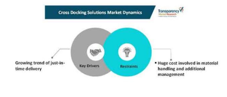
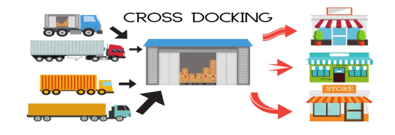
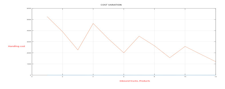
Retail supply chains are intended to empower effectiveness, speed, and cost-savings, guaranteeing that items get to the end client brilliantly, giving rise to the new logistic strategy of cross-docking. Cross-docking popularity depends heavily on properly executing operational-level policies like assigning doors to trucks or handling resources to doors. This paper proposes a linear programming model based on door-to-storage assignment. The model aims to optimize the material handling cost within a cross-dock when goods are unloaded and transferred from the dock area to the storage area. A fraction of the products unloaded at the incoming gates is assigned to different storage zones depending on their demand frequency and the loading sequence. Numerical example considering a varying number of inbound cars, doors, products, and storage areas is analyzed, and the result proves that the cost can be minimized or savings can be intensified based on the feasibility of the research problem. The result explains that a variation in the number of inbound trucks, product quantity, and per-pallet handling prices influences the net material handling cost. However, it remains unaffected by the alteration in the number of material handling resources. The result also verifies that applying direct transfer of product through cross-docking is economical as fewer products in storage reduce the handling cost.
Citation: Taniya Mukherjee, Isha Sangal, Biswajit Sarkar, Qais Ahmed Almaamari. Logistic models to minimize the material handling cost within a cross-dock[J]. Mathematical Biosciences and Engineering, 2023, 20(2): 3099-3119. doi: 10.3934/mbe.2023146
Retail supply chains are intended to empower effectiveness, speed, and cost-savings, guaranteeing that items get to the end client brilliantly, giving rise to the new logistic strategy of cross-docking. Cross-docking popularity depends heavily on properly executing operational-level policies like assigning doors to trucks or handling resources to doors. This paper proposes a linear programming model based on door-to-storage assignment. The model aims to optimize the material handling cost within a cross-dock when goods are unloaded and transferred from the dock area to the storage area. A fraction of the products unloaded at the incoming gates is assigned to different storage zones depending on their demand frequency and the loading sequence. Numerical example considering a varying number of inbound cars, doors, products, and storage areas is analyzed, and the result proves that the cost can be minimized or savings can be intensified based on the feasibility of the research problem. The result explains that a variation in the number of inbound trucks, product quantity, and per-pallet handling prices influences the net material handling cost. However, it remains unaffected by the alteration in the number of material handling resources. The result also verifies that applying direct transfer of product through cross-docking is economical as fewer products in storage reduce the handling cost.

| [1] |
A. Ahmed, M. R. H. Alzgool, Z. Abro, U. Ahmed, U. Memon, Understanding the nexus of intellectual, social and psychological capital towards business innovation through critical insights from organizational culture, Humanit. Soc. Sci. Rev., 7 (2019), 1082–1086. https://doi.org/10.18510/hssr.2019.75144 doi: 10.18510/hssr.2019.75144

|
| [2] |
O. Y. M. Al-Rawi, T. Mukherjee, Application of linear programming in optimizing labour scheduling, J. Math. Financ., 9 (2019), 272–285. https://doi.org/10.4236/jmf.2019.93016 doi: 10.4236/jmf.2019.93016
|
| [3] | B. Oryani, A. Moridian, B. Sarkar, S. Rezania, H. Kamyab, M. K. Khan, Assessing the financial rеsоurсе curse hypothesis in Iran: Thе nоvеl dynаmiс АRDL approach, Resour. Policy, 78 (2022), p. 102899. https://doi.org/10.1016/j.resourpol.2022.102899 |
| [4] |
F. H. Staudt, G. Alpan, M. Di Mascolo, C. M. T. Rodriguez, Warehouse performance measurement: a literature review, Int. J. Prod. Res., 53 (2015), 5524–5544. https://doi.org/10.1080/00207543.2015.1030466 doi: 10.1080/00207543.2015.1030466
|
| [5] |
B. Sarkar, B. K. Dey, M. Sarkar, S. J. Kim, A smart production system with an autonomation technology and dual channel retailing, Comput. Ind. Eng., 173 (2022), 108607. https://doi.org/10.1016/j.cie.2022.108607 doi: 10.1016/j.cie.2022.108607
|
| [6] |
M. Kaviyani, S. Ghodsypour, M. Hajiaghaei-Keshteli, Impact of Adopting Quick Response and Agility on Supply Chain Competition with Strategic Customer Behavior, Sci. Iran., (2020). https://doi.org/10.24200/sci.2020.53691.3366 doi: 10.24200/sci.2020.53691.3366
|
| [7] |
A. Sarkar, R. Guchhait, B. Sarkar, Application of the artificial neural network with multithreading within an inventory model under uncertainty and inflation, Int. J. Fuzzy Syst., 24 (2022), 2318–2332. https://doi.org/10.1007/s40815-022-01276-1 doi: 10.1007/s40815-022-01276-1
|
| [8] |
S. V. S. Padiyar, Vandana, N. Bhagat, S. R. Singh, B. Sarkar, Joint replenishment strategy for deteriorating multi-item through multi-echelon supply chain model with imperfect production under imprecise and inflationary environment, RAIRO-Oper. Res., 56 (2022), 3071–3096. https://doi.org/10.1051/ro/2022071 doi: 10.1051/ro/2022071
|
| [9] |
A. Mondal, S. Pareek, K. Chaudhuri, A. Bera, R. K. Bachar, B. Sarkar, Technology license sharing strategy for remanufacturing industries under a closer-loop supply chain management bonding, RAIRO-Oper. Res., 56 (2022), 3017–3045. https://doi.org/10.1051/ro/2022058 doi: 10.1051/ro/2022058
|
| [10] |
B. Sarkar, S. Kar, K. Basu, R. Guchhait, A sustainable managerial decision-making problem for a substitutable product in a dual-channel under carbon tax policy, Comput. Ind. Eng., 172 (2022), 108635. https://doi.org/10.1016/j.cie.2022.108635 doi: 10.1016/j.cie.2022.108635
|
| [11] |
S. Hota, S. Ghosh, B. Sarkar, Involvement of smart technologies in an advanced supply chain management to solve unreliability under distribution robust approach, AIMS Environ. Sci., 9 (2022), 461–492. https://doi.org/10.3934/environsci.2022028 doi: 10.3934/environsci.2022028
|
| [12] |
B. Sarkar, D. Takeyeva, R. Guchhait, M. Sarkar, Optimized radio-frequency identification system for different warehouse shapes, Knowledge-Based Syst., 258 (2022), 109811. https://doi.org/10.1016/j.knosys.2022.109811 doi: 10.1016/j.knosys.2022.109811
|
| [13] |
R. K. Bachar, S. Bhuniya, S. K. Ghosh, B. Sarkar, Sustainable green production model considering variable demand, partial outsourcing, and rework, AIMS Environ. Sci., 9 (2022), 325–353. https://doi.org/10.3934/environsci.2022022 doi: 10.3934/environsci.2022022
|
| [14] |
B. Shaw, I. Sangal, B. Sarkar, Reduction of greenhouse gas emissions in an imperfect production process under breakdown consideration, AIMS Environ. Sci., 9 (2022), 658–691. https://doi.org/10.3934/environsci.2022038 doi: 10.3934/environsci.2022038
|
| [15] |
S. Kumar, M. Sigroha, K. Kumar, B. Sarkar, Manufacturing/remanufacturing based supply chain management under advertisements and carbon emissions process, RAIRO-Oper. Res., 56 (2022), 831–851.[Online]. Available: https://doi.org/10.1051/ro/2021189 doi: 10.1051/ro/2021189
|
| [16] |
S. Hota, S. Ghosh, B. Sarkar, A solution to the transportation hazard problem in a supply chain with an unreliable manufacturer, AIMS Environ. Sci., 9 (2022), 354–380. https://doi.org/10.3934/environsci.2022023 doi: 10.3934/environsci.2022023
|
| [17] |
G. Maity, V. F. Yu, S. K. Roy, Optimum Intervention in Transportation Networks Using Multimodal System under Fuzzy Stochastic Environment, J. Adv. Transp., 2022 (2022), 3997396. https://doi.org/10.1155/2022/3997396 doi: 10.1155/2022/3997396
|
| [18] |
B. Sarkar, B. Ganguly, S. Pareek, L. E. Cárdenas-Barrón, A three-echelon green supply chain management for biodegradable products with three transportation modes, Comput. Ind. Eng., 174 (2022), 108727. https://doi.org/10.1016/j.cie.2022.108727 doi: 10.1016/j.cie.2022.108727
|
| [19] |
M. Mishra, S. K. Ghosh, B. Sarkar, Maintaining energy efficiencies and reducing carbon emissions under a sustainable supply chain management, AIMS Environ. Sci., 9 (2022), 603–635. https://doi.org/10.3934/environsci.2022036 doi: 10.3934/environsci.2022036
|
| [20] |
A.-L. Ladier, G. Alpan, Cross-docking operations: Current research versus industry practice, Omega, 62 (2016), 145–162. https://doi.org/10.1016/j.omega.2015.09.006 doi: 10.1016/j.omega.2015.09.006
|
| [21] | S. C. Corp, Cross-docking Trend Report, Whitepaper Series, Saddle Creek Corp: Lakeland, FL, USA, 2011. Available: http://www.distributiongroup.com/articles/070111DCMwe.pdf |
| [22] |
F. Essghaier, H. Allaoui, G. Goncalves, Truck to door assignment in a shared cross-dock under uncertainty, Expert Syst. Appl., 182 (2021), 114889. https://doi.org/10.1016/j.eswa.2021.114889 doi: 10.1016/j.eswa.2021.114889
|
| [23] |
P. Bodnar, K. Azadeh, R. De Koster, Scheduling trucks in a cross-dock with mixed service mode dock doors, Transp. Sci., 51 (2015). https://doi.org/10.1287/trsc.2015.0612 doi: 10.1287/trsc.2015.0612
|
| [24] |
J. Van Belle, P. Valckenaers, D. Cattrysse, Cross-docking: State of the art, Omega, 40 (2012), 827–846. https://doi.org/10.1016/j.omega.2012.01.005 doi: 10.1016/j.omega.2012.01.005
|
| [25] |
S. Ambroszkiewicz, S. Bylka, Relatively optimal policies for stock management in a supply chain with option for inventory space limitation, Appl. Math. model., 114 (2023), 291–317. https://doi.org/10.1016/j.apm.2022.09.033 doi: 10.1016/j.apm.2022.09.033
|
| [26] |
A. (Arsalan) Ardakani, J. Fei, A systematic literature review on uncertainties in cross-docking operations, Mod. Supply Chain Res. Appl., 2 (2020), 2–22. https://doi.org/10.1108/MSCRA-04-2019-0011 doi: 10.1108/MSCRA-04-2019-0011
|
| [27] |
M. F. Monaco, M. Sammarra, Managing loading and discharging operations at cross-docking terminals, Procedia Manuf., 42 (2020), 475–482.https://doi.org/10.1016/j.promfg.2020.02.045 doi: 10.1016/j.promfg.2020.02.045
|
| [28] |
K. Stephan, N. Boysen, Cross-docking, J. Manag. Control, 22 (2011), 129. https://doi.org/10.1007/s00187-011-0124-9 doi: 10.1007/s00187-011-0124-9
|
| [29] |
P. Buijs, I. F. A. Vis, H. J. Carlo, Synchronization in cross-docking networks: A research classification and framework, Eur. J. Oper. Res., 239 (2014), 593–608. https://doi.org/10.1016/j.ejor.2014.03.012 doi: 10.1016/j.ejor.2014.03.012
|
| [30] |
W. Wisittipanich, T. Irohara, P. Hengmeechai, Truck scheduling problems in the cross docking network, Int. J. Logist. Syst. Manag., 33 (2019), 420. https://doi.org/10.1504/IJLSM.2019.101164 doi: 10.1504/IJLSM.2019.101164
|
| [31] |
P. B. Castellucci, A. M. Costa, F. Toledo, Network scheduling problem with cross-docking and loading constraints, Comput. Oper. Res., 132 (2021), 105271. https://doi.org/10.1016/j.cor.2021.105271 doi: 10.1016/j.cor.2021.105271
|
| [32] |
G. Tadumadze, N. Boysen, S. Emde, F. Weidinger, Integrated truck and workforce scheduling to accelerate the unloading of trucks, Eur. J. Oper. Res., 278 (2019), 343–362. https://doi.org/10.1016/j.ejor.2019.04.024 doi: 10.1016/j.ejor.2019.04.024
|
| [33] |
A. M. Fathollahi-Fard, M. Ranjbar-Bourani, N. Cheikhrouhou, M. Hajiaghaei-Keshteli, Novel modifications of social engineering optimizer to solve a truck scheduling problem in a cross-docking system, Comput. Ind. Eng., 137 (2019), 106103. https://doi.org/10.1016/j.cie.2019.106103 doi: 10.1016/j.cie.2019.106103
|
| [34] |
A. Golshahi-Roudbaneh, M. Hajiaghaei-Keshteli, M. M. Paydar, Developing a lower bound and strong heuristics for a truck scheduling problem in a cross-docking center, Knowledge-Based Syst., 129 (2017), 17–38. https://doi.org/10.1016/j.knosys.2017.05.006 doi: 10.1016/j.knosys.2017.05.006
|
| [35] |
M. A. Dulebenets, A diploid evolutionary algorithm for sustainable truck scheduling at a cross-docking facility, Sustain., 10 (2018), 1333.https://doi.org/10.3390/su10051333 doi: 10.3390/su10051333
|
| [36] |
M. A. Dulebenets, A comprehensive evaluation of weak and strong mutation mechanisms in evolutionary algorithms for truck scheduling at cross-docking terminals, IEEE Access, 6 (2018), 65635–65650. https://doi.org/10.1109/ACCESS.2018.2874439 doi: 10.1109/ACCESS.2018.2874439
|
| [37] |
M. A. Dulebenets, An adaptive polyploid memetic algorithm for scheduling trucks at a cross-docking terminal, Inf. Sci. (Ny)., 565 (2021), 390–421. https://doi.org/10.1016/j.ins.2021.02.039 doi: 10.1016/j.ins.2021.02.039
|
| [38] |
M. A. Dulebenets, A delayed start parallel evolutionary algorithm for just-in-time truck scheduling at a cross-docking facility, Int. J. Prod. Econ., 212 (2019), 236–258. https://doi.org/10.1016/j.ijpe.2019.02.017 doi: 10.1016/j.ijpe.2019.02.017
|
| [39] |
O. Theophilus, M. A. Dulebenets, J. Pasha, O. F. Abioye, M. Kavoosi, Truck scheduling at cross-docking terminals: A follow-up state-of-the-art review, Sustain., 11 (2019), 5245. https://doi.org/10.3390/su11195245 doi: 10.3390/su11195245
|
| [40] |
S. Mousavi, B. Vahdani, A robust approach to multiple vehicle location-routing problems with time windows for optimization of cross-docking under uncertainty, J. Intell. Fuzzy Syst., 32 (2017), 49–62. http://dx.doi.org/10.3233/JIFS-151050 doi: 10.3233/JIFS-151050
|
| [41] |
X. Zhang, J. Li, Z. Yang, X. Wang, Collaborative optimization for loading operation planning and vessel traffic scheduling in dry bulk ports, Adv. Eng. Informatics, 51 (2022), 101489. https://doi.org/10.1016/j.aei.2021.101489 doi: 10.1016/j.aei.2021.101489
|
| [42] |
O. Theophilus, M. A. Dulebenets, J. Pasha, Y. yip Lau, A. M. Fathollahi-Fard, A. Mazaheri, Truck scheduling optimization at a cold-chain cross-docking terminal with product perishability considerations, Comput. Ind. Eng., 156 (2021), 107240. https://doi.org/10.1016/j.cie.2021.107240 doi: 10.1016/j.cie.2021.107240
|
| [43] |
A. Golshahi-Roudbaneh, M. Hajiaghaei-Keshteli, M. M. Paydar, Cross-dock scheduling considering time windows and deadline for truck departures, Sci. Iran., 28 (2021), 532–546. https://doi.org/10.24200/sci.2019.52662.2824 doi: 10.24200/sci.2019.52662.2824
|
| [44] |
F. Pan, W. Zhou, T. Fan, S. Li, C. Zhang, Deterioration rate variation risk for sustainable cross-docking service operations, Int. J. Prod. Econ., 232 (2021), 107932. https://doi.org/10.1016/j.ijpe.2020.107932 doi: 10.1016/j.ijpe.2020.107932
|
| [45] |
F. Zheng, Y. Pang, Y. Xu, M. Liu, Heuristic algorithms for truck scheduling of cross-docking operations in cold-chain logistics, Int. J. Prod. Res., 59 (2021), 6579–6600. https://doi.org/10.1080/00207543.2020.1821118 doi: 10.1080/00207543.2020.1821118
|
| [46] |
L. C. Soares, E. Ferneda, H. A. do Prado, Transportation and logistics observatories: Guidelines for a conceptual model, Transp. Res. Interdiscip. Perspect., 16 (2022), 100682. https://doi.org/10.1016/j.trip.2022.100682 doi: 10.1016/j.trip.2022.100682
|
| [47] |
M. Forkan, M. M. Rizvi, M. A. M. Chowdhury, Multiobjective reverse logistics model for inventory management with environmental impacts: An application in industry, Intell. Syst. with Appl., 14 (2022), 200078. https://doi.org/10.1016/j.iswa.2022.200078 doi: 10.1016/j.iswa.2022.200078
|
| [48] |
Y. Idel Mahjoub, E. houcine Chakir El-Alaoui, A. Nait-Sidi-Moh, Logistic network modeling and optimization: An approach based on (max, +) algebra and coloured Petri nets, Comput. Ind. Eng., 158 (2021), 107341. https://doi.org/10.1016/j.cie.2021.107341 doi: 10.1016/j.cie.2021.107341
|
| [49] |
N. Boysen, M. Fliedner, Cross dock scheduling: Classification, literature review and research agenda, Omega, 38 (2010), 413–422. https://doi.org/10.1016/j.omega.2009.10.008 doi: 10.1016/j.omega.2009.10.008
|
| [50] |
S. Pan, D. Trentesaux, D. McFarlane, B. Montreuil, E. Ballot, G. Q. Huang, Digital interoperability in logistics and supply chain management: state-of-the-art and research avenues towards physical internet, Comput. Ind., 128 (2021), 103435. https://doi.org/10.1016/j.compind.2021.103435 doi: 10.1016/j.compind.2021.103435
|
| [51] |
T. Chargui, A.-L. Ladier, A. Bekrar, S. Pan, D. Trentesaux, Towards designing and operating physical internet cross-docks: Problem specifications and research perspectives, Omega, 111 (2022), 102641. https://doi.org/10.1016/j.omega.2022.102641 doi: 10.1016/j.omega.2022.102641
|
| [52] | T. Mukherjee, I. Sangal, B. Sarkar, T. M. Alkadash, Mathematical estimation for maximum flow of goods within a cross-dock to reduce inventory, 19 (2022), 13710–13731. https://doi.org/10.3934/mbe.2022639 |
| [53] |
G. Vieira, G. Pasa, M. Borsa, G. S. Milan, A. Pandolfo, Materials handling management:A case study, J. Oper. Supply Chain Manag., 4 (2011), 19. https://doi.org/10.12660/joscmv4n2p19-30 doi: 10.12660/joscmv4n2p19-30
|
| [54] | S. K. Das, M. Pervin, S. K. Roy, G. W. Weber, Multi-objective solid transportation-location problem with variable carbon emission in inventory management: a hybrid approach, Ann. Oper. Res., (2021), 1–27. https://doi.org/10.1007/s10479-020-03809-z |
| [55] |
M. Cherkesly, T. Gschwind, The pickup and delivery problem with time windows, multiple stacks, and handling operations, Eur. J. Oper. Res., 301(2022), 647–666. https://doi.org/10.1016/j.ejor.2021.11.021 doi: 10.1016/j.ejor.2021.11.021
|
| [56] |
M. Bertolini, D. Mezzogori, M. Neroni, F. Zammori, A dynamic operative framework for allocation in automated storage and retrieval systems, Expert Syst. Appl., 213 (2023), 118940. https://doi.org/10.1016/j.eswa.2022.118940 doi: 10.1016/j.eswa.2022.118940
|
| [57] | İ. Küç ükoğlu, The effects of crossdock shapes on material handling costs, Int. J. Comput. Eng. Res., 10 (2016), 2250–3005. |
| [58] |
W. Nassief, I. Contreras, R. As'ad, A mixed-integer programming formulation and Lagrangean relaxation for the cross-dock door assignment problem, Int. J. Prod. Res., 54 (2016), 494–508. https://doi.org/10.1080/00207543.2014.1003664 doi: 10.1080/00207543.2014.1003664
|
| [59] | L. Zhang, Optimization and simulation of a cross-docking terminal, PhD Thesis, Ecole Centrale de Lille, France, 2016. |
| [60] |
C. Serrano, X. Delorme, A. Dolgui, Cross-dock distribution and operation planning for overseas delivery consolidation: A case study in the automotive industry, CIRP J. Manuf. Sci. Technol., 33 (2021), 71–81. https://doi.org/10.1016/j.cirpj.2021.02.007 doi: 10.1016/j.cirpj.2021.02.007
|
| [61] |
S. Shahram fard, B. Vahdani, Assignment and scheduling trucks in cross-docking system with energy consumption consideration and trucks queuing, J. Clean. Prod., 213 (2019), 21–41. https://doi.org/10.1016/j.jclepro.2018.12.106 doi: 10.1016/j.jclepro.2018.12.106
|
| [62] |
Q. Fabry, A. Agnetis, L. Berghman, C. Briand, Complexity of flow time minimization in a crossdock truck scheduling problem with asymmetric handover relations, Oper. Res. Lett., 50 (2022), 50–56. https://doi.org/10.1016/j.orl.2021.12.004 doi: 10.1016/j.orl.2021.12.004
|
| [63] |
W. Yu, P. J. Egbelu, Scheduling of inbound and outbound trucks in cross docking systems with temporary storage, Eur. J. Oper. Res., 184 (2008), 377–396. https://doi.org/10.1016/j.ejor.2006.10.047 doi: 10.1016/j.ejor.2006.10.047
|
| [64] |
A. Fumi, L. Scarabotti, M. M. Schiraldi, Minimizing warehouse space with a dedicated storage policy, Int. J. Eng. Bus. Manag., 5 (2013), 21. https://doi.org/10.5772/56756 doi: 10.5772/56756
|
| [65] |
A. S. Dijkstra, K. J. Roodbergen, Exact route-length formulas and a storage location assignment heuristic for picker-to-parts warehouses, Transp. Res. Part E Logist. Transp. Rev., 102 (2017), 38–59. https://doi.org/10.1016/j.tre.2017.04.003 doi: 10.1016/j.tre.2017.04.003
|
| [66] |
E. Charris, J. Rojas-Reyes, J. Montoya-Torres, The storage location assignment problem: A literature review, Int. J. Ind. Eng. Comput., 10 (2018), 199–224. https://doi.org/10.5267/j.ijiec.2018.8.001 doi: 10.5267/j.ijiec.2018.8.001
|
| [67] |
N. Zaerpour, Y. Yu, R. De Koster, Storing fresh produce for fast retrieval in an automated compact cross-dock system, Prod. Oper. Manag., 24 (2014). https://doi.org/10.1111/poms.12321 doi: 10.1111/poms.12321
|
| [68] |
A. Silva, K. J. Roodbergen, L. C. Coelho, M. Darvish, Estimating optimal ABC zone sizes in manual warehouses, Int. J. Prod. Econ., 252 (2022), 108579. https://doi.org/10.1016/j.ijpe.2022.108579 doi: 10.1016/j.ijpe.2022.108579
|
| [69] |
N. Zaerpour, R. De Koster, Y. Yu, Storage policies and optimal shape of a storage system, Int. J. Prod. Res., 51 (2013). https://doi.org/10.1080/00207543.2013.774502 doi: 10.1080/00207543.2013.774502
|
| [70] |
D. Sun, Y. Meng, L. Tang, J. Liu, B. Huang, J. Yang, Storage space allocation problem at inland bulk material stockyard, Transp. Res. Part E Logist. Transp. Rev., 134 (2020), 101856. https://doi.org/10.1016/j.tre.2020.101856 doi: 10.1016/j.tre.2020.101856
|
| [71] | Y. Wooyeon, Operational strategies for cross docking systems, Phd Thesis, Iowa State University, Ames, Iowa, 2002. https://doi.org/10.31274/rtd-180813-11026 |

Figures(4) / Tables(3)

Taniya Mukherjee, Isha Sangal, Biswajit Sarkar, Qais Ahmed Almaamari. Logistic models to minimize the material handling cost within a cross-dock[J]. Mathematical Biosciences and Engineering, 2023, 20(2): 3099-3119. doi: 10.3934/mbe.2023146


 DownLoad: