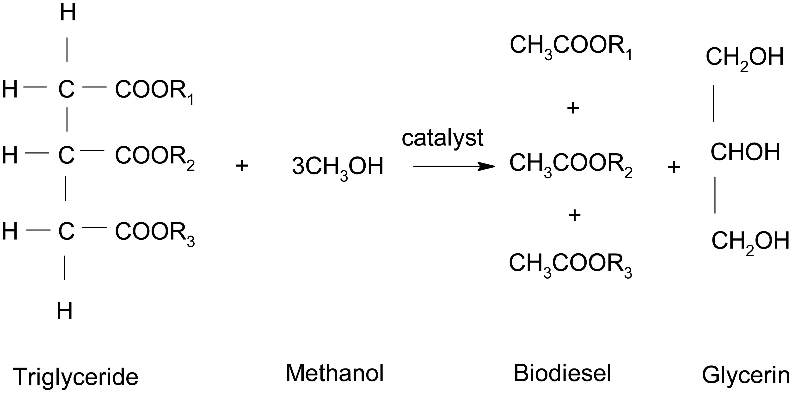
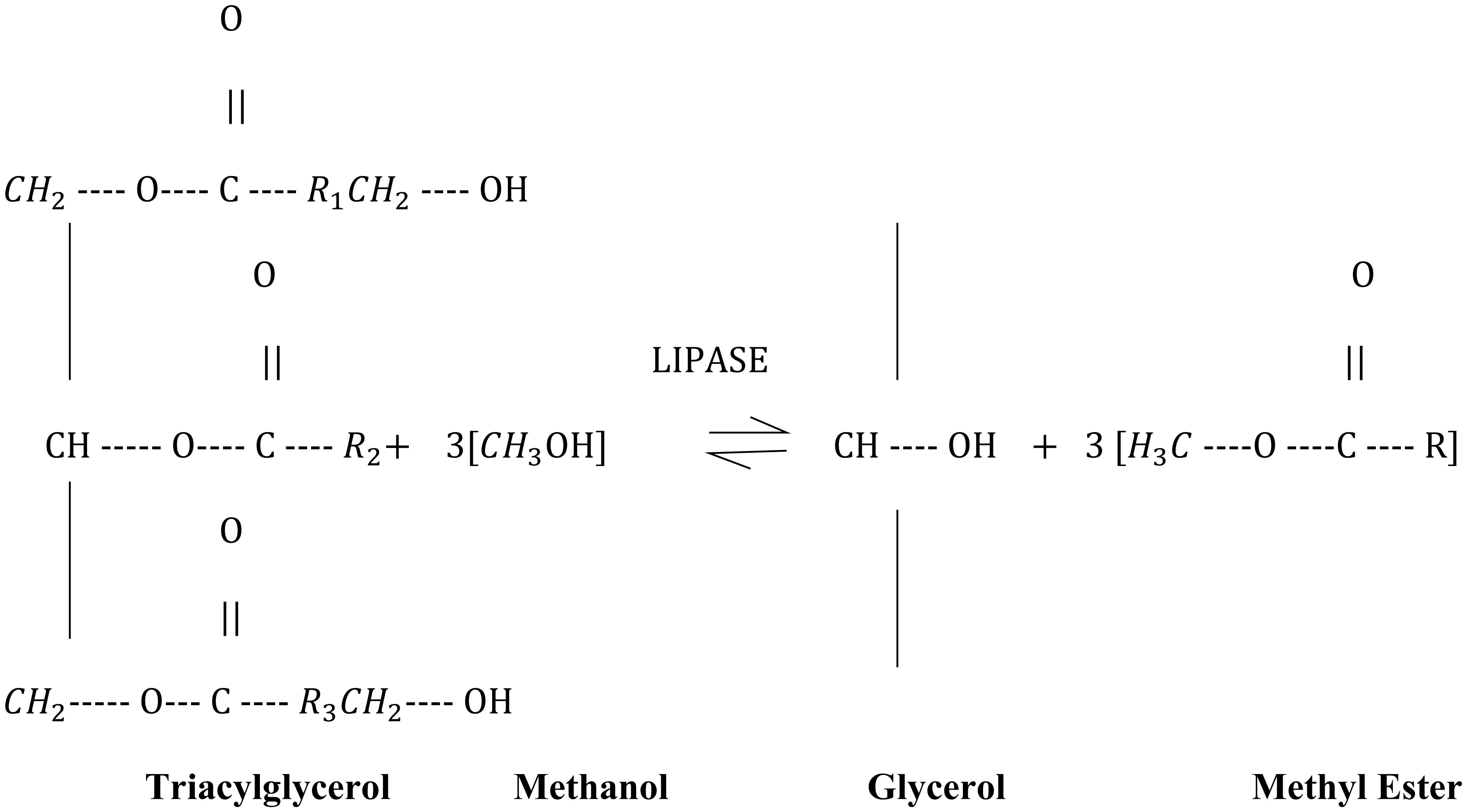
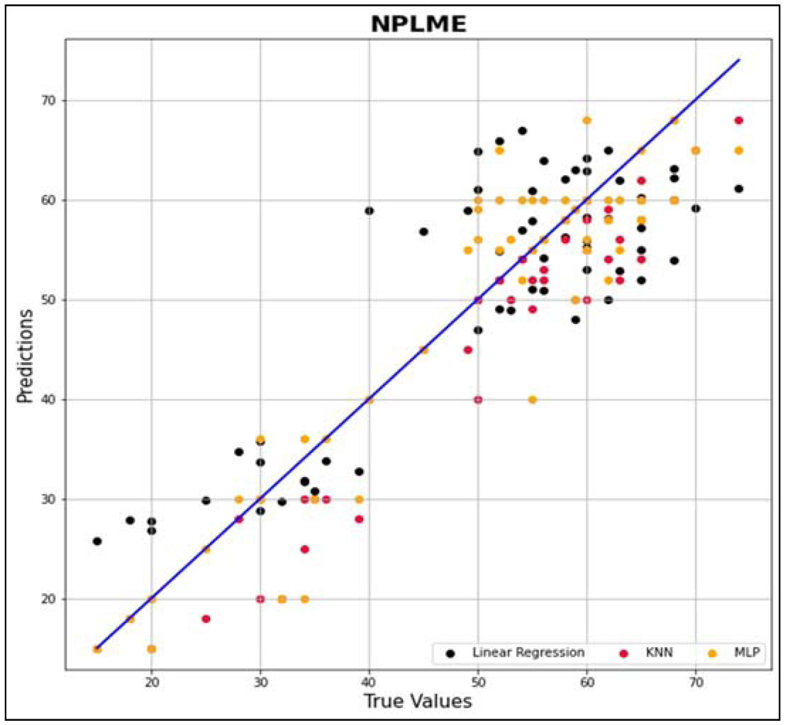
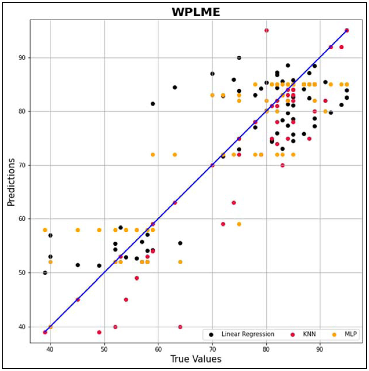
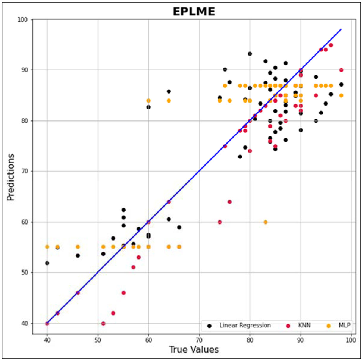
In this research work, various machine learning models such as linear regression (LR), KNN and MLP were created to predict the optimized synthesis of biodiesel from pre-treated and non-treated Linseed oil in base transesterification reaction mode. Three input parameters were included for modelling, reaction time, catalyst concentrated ion, and methanol/oil-molar ratio. In biodiesel transesterification reaction 180 samples run with non-Pre-treated Linseed Methyl Ester (NPLME), Water Pre-treated Linseed Methyl Ester (WPLME) and Enzymatic Pre-treated Linseed Methyl Ester (EPLME) oil as feed stocks and optimized parameters are find out for maximum biodiesel yield to be 8:1 molar ratio, 0.4% weight catalyst, 60 °C reaction temperature.To test the technique, R2 and MAPE parameters were used. The average R2 values for linear regression, KNN, and MLP are 0.7030, 0.8554 and 0.7864 respectively. Moreover, the average MAPE values for these models are 11.1886, 6.0873 and 8.0669 respectively. Hence, it is observed that the KNN model outperforms other models with higher accuracy and low MAPE score.
Citation: Sunil Gautam, Sangeeta Kanakraj, Azriel Henry. Computational approach using machine learning modelling for optimization of transesterification process for linseed biodiesel production[J]. AIMS Bioengineering, 2022, 9(4): 319-336. doi: 10.3934/bioeng.2022023
In this research work, various machine learning models such as linear regression (LR), KNN and MLP were created to predict the optimized synthesis of biodiesel from pre-treated and non-treated Linseed oil in base transesterification reaction mode. Three input parameters were included for modelling, reaction time, catalyst concentrated ion, and methanol/oil-molar ratio. In biodiesel transesterification reaction 180 samples run with non-Pre-treated Linseed Methyl Ester (NPLME), Water Pre-treated Linseed Methyl Ester (WPLME) and Enzymatic Pre-treated Linseed Methyl Ester (EPLME) oil as feed stocks and optimized parameters are find out for maximum biodiesel yield to be 8:1 molar ratio, 0.4% weight catalyst, 60 °C reaction temperature.To test the technique, R2 and MAPE parameters were used. The average R2 values for linear regression, KNN, and MLP are 0.7030, 0.8554 and 0.7864 respectively. Moreover, the average MAPE values for these models are 11.1886, 6.0873 and 8.0669 respectively. Hence, it is observed that the KNN model outperforms other models with higher accuracy and low MAPE score.

| [1] | McDonnell K, Ward S, Leahy J, et al. (1999) Properties of rapeseed oil for use as a diesel fuel extender. J Am Oil Chem Soc 76: 539-543. https://doi.org/10.1007/s11746-999-0001-y |
| [2] | Zufarov O, Schmidt S, Sekretar S (2008) Degumming of rapseed and sunflower oils. Acta Chemica Slovaca 1: 321-328. |
| [3] | Fan X (2008) Optimization of biodiesel production from crude cottonseed oil and waste vegetable oil: Conventional and ultrasonic irradiation methods [PhD thesis]. USA: Clemson University. |
| [4] | Ragit S (2011) Process standardization, characterization and experimental investigation on the performance of biodiesel fuelled C.I. engine [PhD thesis]. Patiala: Thapar university. |
| [5] | Rashid U, Anwar F, Jamil A, et al. (2010) Jatropha curcas seed oil as a viable source for biodiesel. Pak J Bot 42: 575-582. |
| [6] | Navindgi M, Dutta M, Kumar B (2012) Performance evaluation, emission characteristics and economic analysis of four non-edible straight vegetable oils on a single cylinder CI engine APRN. J Eng Appl Sci 7: 173-179. |
| [7] | Giva S, Abdullah L, Adam N (2010) Investigating Egusi (Citrullus Colocynthis L.) seed oil as potential biodiesel feedstock. Energies 3: 607-618. https://doi.org/10.3390/en3040607 |
| [8] | Heiden R (1996) Analytical methodologies for the determination of biodiesel ester purity determination of total methyl esters. National Biodiesel board . |
| [9] | Sharma Y, Singh B, Upadhyay S (2008) Advanced in development and characterization of biodiesel: A review. Fuel 87: 2355-2373. https://doi.org/10.1016/j.fuel.2008.01.014 |
| [10] | Leung DYC, Guo Y (2006) Transesterification of neat and used frying oil: optimization for biodiesel production. Fuel Process Technol 87: 883-890. https://doi.org/10.1016/j.fuproc.2006.06.003 |
| [11] | Somnuk K, Smithmait P, Prateepchaikul G (2012) Feasibility of using ultrasound assisted biodiesel production from degummed deacidifies mixed crude palm oil using small scale Circulation. Agric Nat Reso 46: 662-669. |
| [12] | Saqib M, Mumtaz MW, Mahmood A, et al. (2012) Optimized biodiesel production and environmental assessment produced biodiesel. Biotechnol Bioprocess Eng 17: 617-623. https://doi.org/10.1007/s12257-011-0569-6 |
| [13] | Ramadhas AS, Jayaraj S, Muraleedharan C (2005) Biodiesel production from high FFA rubber seed oil. Fuel 84: 335-340. https://doi.org/10.1016/j.fuel.2004.09.016 |
| [14] | Peddroso L, Ferreira J, Falco J, et al. PortugalBiodiesel alternative (2020). Available from https://ec.europa.eu/environment/nature/natura2000/management/docs/Annex%20report.pdf. |
| [15] | Srivastava A, Prasad R (2000) Triglycerides-based diesel fuels. Renew Sust Energy Rev 4: 111-133. https://doi.org/10.1016/S1364-0321(99)00013-1 |
| [16] | Bari S, Lim T, Yu C (2002) Effects of preheating crude palm oil (CPO) on injection system, performance and emission of a diesel engine. Renew Energy 27: 171-181. https://doi.org/10.1016/S0960-1481(02)00010-1 |
| [17] | Pehan S, Jerman M, Kegl M, et al. (2009) Biodiesel influence on tribology characteristics of a diesel engine. Fuel 88: 970-979. https://doi.org/10.1016/j.fuel.2008.11.027 |
| [18] | Devi J, Pachwania S (2018) Recent advancements in DNA interaction studies of organotin (IV) complexes. Inorg Chem Commun 91: 44-62. https://doi.org/10.1016/j.inoche.2018.03.012 |
| [19] | Tariq M, Ali S, Muhammad N, et al. (2014) Biological screening, DNA interaction studies, and catalytic activity of organotin (IV) 2-(4-ethylbenzylidene) butanoic acid derivatives: synthesis, spectroscopic characterization, and X-ray structure. J Coord Chem 67: 323-340. https://doi.org/10.1080/00958972.2014.884217 |
| [20] | Rathore V, Giridhar M (2007) Synthesis of bio-diesel from edible and non-edible oils in supercritical alcohols and enzymatic synthesis in supercritical carbon dioxide. Fuel 86: 2650-2659. https://doi.org/10.1016/j.fuel.2007.03.014 |
| [21] | Dixit S, Rehman A (2012) Linseed oil as a potential resource for bio-diesel: a review. Renew Sust Energy Rev 16: 4415-4421. https://doi.org/10.1016/j.rser.2012.04.042 |
| [22] | Wilson P (2010) Biodiesel production from Jatropha curcas: A review. Sci Res Essays 5: 1796-1808. |
| [23] | Gupta KK, Rehman A, Sarviya RM (2010) Evaluation of soya bio-diesel as a gas turbine fuel. Iran J Energy Environ 1: 205-210. |
| [24] | Tiwari P, Kumar R, Garg S (2006) Transesterification, modeling and simulation of batch kinetics of non-edible vegetable oils for biodiesel production. Annu Alche Meet . San Francisco: . |
| [25] | Agarwal A (2007) Biofuels (alcohols and biodiesel) applications as fuels for internal combustion engines. Prog Energy Combust Sci 33: 233-271. https://doi.org/10.1016/j.pecs.2006.08.003 |
| [26] | Rao Y, Voleti R, Raju A (2009) Experimental investigations on jatropha biodiesel and additive in diesel engine YV Hanumantha Rao1, Ram Sudheer Voleti1, AV Sitarama Raju2 and P. Nageswara Reddy3. Indian J Sci Technol 2: 25-31. https://doi.org/10.17485/ijst/2009/v2i4.13 |
| [27] | Chatterjee M, Mitra J, Saha S (2010) Bio-diesel: Production through the Enzymatic Route [MD thesis]. India: Jadavpur University. |
| [28] | Mathiyazhagan M, Ganapathi A, Jaganath B, et al. (2011) Production of biodiesel from non-edible plant oils having high FFA content. Int J Chem Environ Eng 2: 119-122. |
| [29] | Raheman H, Phadatare AG (2003) Karanja esterified oil an alternative renewable fuel for diesel engines in controlling air pollution. Bioenergy News 7: 17-23. |
| [30] | Srinivas P, Gopalakrishnan KV (1991) Vegetable oils and their methyl esters as fuels for diesel engines. Indian J Technol 29: 292-297. |
| [31] | Shereena KM, Thangaraj T (2009) Bio-diesel: an alternative fuel produced from vegetable oils by transesterification. Elec J Biol 5: 67-74. |
| [32] | Gondra Z Study of factors influencing the quality and yield of biodiesel produced by transesterification of vegetable oils (2009). |
| [33] | Padhi S, Singh R (2010) Optimization of esterification and transesterification of Mahua (Madhuca Indica) oil for production of biodiesel. J Chem Pharm Res 2: 599-608. |
| [34] | Naik M, Meher, L, Naik S, et al. (2008) Production of biodiesel from high free fatty acid Karanja (Pongamia pinnata) oil. Biomass Bioenergy 32: 354-357. https://doi.org/10.1016/j.biombioe.2007.10.006 |
| [35] | Gandhi M, Ramu N, Raj SB (2011) Methyl ester production from Schlichera oleosa. Int J Pharm Sci Res 2: 1244-1250. |
| [36] | Haldar S, Nag A (2008) Utilization of three non-edible vegetable oils for the production of biodiesel catalysed by enzyme. The Open Chem Eng J 2: 79-83. https://doi.org/10.2174/1874123100802010079 |
| [37] | Shah S, Sharma S, Gupta M (2003) Enzymatic transesterification for biodiesel production. IJBB 40: 392-399. |
| [38] | Ju Y, Vali S (2005) Rice bran oil as a potential resource for biodiesel: a review. J Sci Ind Res 64: 866-882. |
| [39] | Helwani Z, Othman M, Aziz N, et al. (2009) Technologies for production of biodiesel focusing on green catalytic techniques: a review. Fuel Process Technol 90: 1502-1514. https://doi.org/10.1016/j.fuproc.2009.07.016 |
| [40] | Bunkakiat K (2006) Continuous production of biodiesel via transesterifi-cation from vegetable oils in supercritical methanol. Energy Fuels 20: 812-817. https://doi.org/10.1021/ef050329b |
| [41] | Kusdiana D, Saka S (2004) Effects of water on biodiesel fuel production by supercritical methanol treatment. Bioresource Technol 91: 289-295. https://doi.org/10.1016/s0960-8524(03)00201-3 |
| [42] | Vera CR, D'Ippolito SA, Pieck CL, et al. Production of biodiesel by a two-step supercritical reaction process with adsorption refining, 2nd Mercosur Congress on Chemical Engineering. Rio de Janeiro (2005)2005: 14-18. |
| [43] | Andualem B, Gessesse A (2012) Methods for refining of brebra (Millettiaferruginea) Oil for the production of biodiesel. World App Sci J 17: 407-413. |
| [44] | Mamilla V, Mllikarjun M, Laxmi G, et al. (2011) Preparation of biodiesel from karanj oil. Int J Energy Eng 1: 94-100. https://doi.org/10.5963/IJEE0102008 |
| [45] | Somnuk K, Smithmaitrie P, Prateepchaikul G (2012) Feasibility of using ultrasound-assisted biodiesel production from degummed-deacidified mixed crude palm oil using small-scale circulation. Agric Nat Res 46: 662-669. |
| [46] | Hossain A, Boyce A, Salleh A, et al. (2010) Impacts of alcohol type, ratio and stirring time on the biodiesel production from waste canola oil. Afr J Agric Res 5: 1851-1859. https://doi.org/10.5897/AJAR09.135 |
| [47] | Freedman B, Pryde E, Mounts T (1984) Variables affecting the yields of fatty esters from transesterified vegetable oils. J Am Oil Chem Soc 61: 1638-1643. https://doi.org/10.1007/BF02541649 |
| [48] | Ramadhas A, Jayaraj S, Muraleedharan C (2005) Biodiesel production from high FFA rubber seed oil. Fuel 84: 335-340. https://doi.org/10.1016/j.fuel.2004.09.016 |
| [49] | Schmidt A, Finan C (2018) Linear regression and the normality assumption. J Clin Epidemiol 98: 146-151. https://doi.org/10.1016/j.jclinepi.2017.12.006 |
| [50] | Katrina W A guide to machine learning algorithms and their applications (2022). Available from: https://www.sas.com/en_us/insights/articles/analytics/machine-learning-algorithms-guide.html. |
| [51] | Yang K, Shahabi C (2007) An efficient k nearest neighbor search for multivariate time series. Inform Comput 205: 65-98. https://doi.org/10.1016/j.ic.2006.08.004 |
| [52] | Baran B (2021) Air quality Index prediction in besiktas district by artificial neural networks and k nearest neighbors. J Eng Sci Design 9: 52-63. https://doi.org/10.21923/jesd.671836 |
| [53] | Li Y, Cao W (2019) An extended multilayer perceptron model using reduced geometric algebra. IEEE Access 7: 129815-129823. https://doi.org/10.1109/ACCESS.2019.2940217 |
| [54] | Sreedharan M, Khedr A, Bannany M (2020) A multi-layer perceptron approach to financial distress prediction with genetic algorithm. Autom Control Comput Sci 54: 475-482. https://doi.org/10.3103/S0146411620060085 |
| [55] | Schmidt A, Finan C (2018) Linear regression and the normality assumption. J Clin Epidemiol 98: 146-151. https://doi.org/10.1016/j.jclinepi.2017.12.006 |
| [56] | Coben D, Colwell D, Macrae S, et al. (2003) Adult numeracy: Review of research and related literature. London: National Research and Development Centre for adult literacy and numeracy. |
| [57] | Chicco D, Warrens MJ, Jurman G (2021) The coefficient of determination R-squared is more informative than SMAPE, MAE, MAPE, MSE and RMSE in regression analysis evaluation. PeerJ Comput Sci 7: e623. https://doi.org/10.7717/peerj-cs.623 |
| [58] | Abdelbasset W, Elkholi S, Opulencia C, et al. (2022) Development of multiple machine-learning computational techniques for optimization of heterogenous catalytic biodiesel production from waste vegetable oil. Arabian J Chem 15: 103843. https://doi.org/10.1016/j.arabjc.2022.103843 |
| [59] | Mathiyazhagan M, Ganapathi A (2011) Factor affecting biodiesel production. Res Plant Biol 1: 1-5. |
| [60] | Singh P, Singh D (2010) Bio-diesel production through the use of different sources and characterization of oils and their esters as the substitute of diesel: a review. Renew Sust Energy Rev 14: 200-216. https://doi.org/10.1016/j.rser.2009.07.017 |
| [61] | Sirajuddin M, Tariq M, Ali S (2015) Organotin (IV) carboxylates as an effective catalyst for the conversion of corn oil into biodiesel. J Organomet Chem 779: 30-38. https://doi.org/10.1016/j.jorganchem.2014.12.019 |
| [62] | Tariq M, Qureshi A, Imran M, et al. (2019) biodiesel-a transesterified product of non-edible castor oil. Rev Roum Chim 64: 1027-1036. https://doi.org/10.33224/rrch/2019.64.12.02 |
| [63] | Tariq M, Qureshi A, Karim S, et al. (2021) Synthesis, characterization and fuel parameters analysis of linseed oil biodiesel using cadmium oxide nanoparticles. Energy 222: 120014. https://doi.org/10.1016/j.energy.2021.120014 |
| [64] | Karthikumar S, Ragavanandham V, Kanagaraj S, et al. (2014) Preparation, characterization and engine performance characteristics of used cooking sunflower oil based bio-fuels for a diesel engine. Adv Mater Res 984: 913-923. https://doi.org/10.4028/www.scientific.net/AMR.984-985.913 |
Figures(7) / Tables(3)

Sunil Gautam, Sangeeta Kanakraj, Azriel Henry. Computational approach using machine learning modelling for optimization of transesterification process for linseed biodiesel production[J]. AIMS Bioengineering, 2022, 9(4): 319-336. doi: 10.3934/bioeng.2022023


 DownLoad: