Walking dynamics for an ascending stair biped robot with telescopic legs and impulse thrust

Jiarui Chen; Aimin Tang; Guanfeng Zhou; Ling Lin; Guirong Jiang; Jiarui Chen; Aimin Tang; Guanfeng Zhou; Ling Lin; Guirong Jiang

doi:10.3934/era.2022208

Electronic Research Archive

2022, Volume 30, Issue 11: 4108-4135. doi: 10.3934/era.2022208

Previous Article Next Article

Research article

Walking dynamics for an ascending stair biped robot with telescopic legs and impulse thrust

1.
School of Mathematics and Computing Science, Guilin University of Electronic Technology, Guilin 541004, China
2.
Library, Guilin University of Electronic Technology, Guilin 541004, China
3.
School of Electronic Engineering and Automation, Guilin University of Electronic Technology, Guilin 541004, China

Received: 27 June 2022 Revised: 16 August 2022 Accepted: 29 August 2022 Published: 19 September 2022

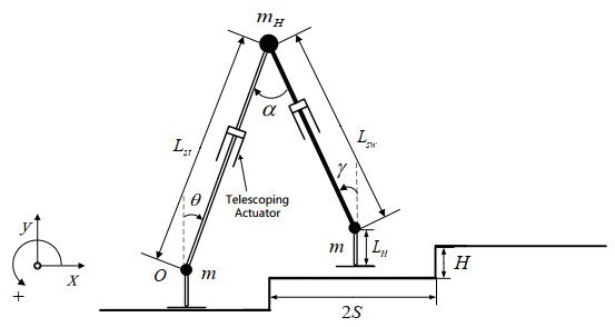
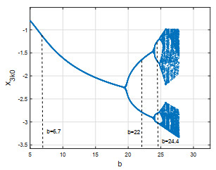
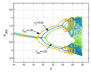
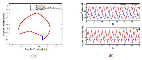
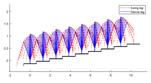
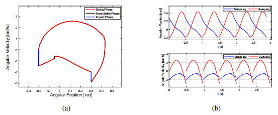
In this study, an ascending stair biped robot model with impulse thrust is presented. The biped robot contains a hip joint and two legs with massless telescoping actuator. Impulse thrust is applied at the ankle joint of robot's stance leg to simulate the forward push-off of the ankle during human walking. The nonlinear ascending stair biped model is linearized and a discrete map is obtained. The conditions for the existence and stability of period-1 gait are obtained by means of this discrete map. The expressions of torques to ensure robot walking are derived and Flip bifurcation is investigated. Numerical simulations, such as phase diagram of period-1, 2, 4 gaits and bifurcation diagram, are given in an example. Theoretical analysis and numerical results obtained in this study provide a theoretical basis for stable walking of ascending stair biped robot with periodic gaits.

Keywords:

Citation: Jiarui Chen, Aimin Tang, Guanfeng Zhou, Ling Lin, Guirong Jiang. Walking dynamics for an ascending stair biped robot with telescopic legs and impulse thrust[J]. Electronic Research Archive, 2022, 30(11): 4108-4135. doi: 10.3934/era.2022208

Related Papers:

[1]	Lisa Bigler, Malgorzata Peszynska, Naren Vohra . Heterogeneous Stefan problem and permafrost models with P0-P0 finite elements and fully implicit monolithic solver. Electronic Research Archive, 2022, 30(4): 1477-1531. doi: 10.3934/era.2022078
[2]	Jianxia He, Qingyan Li . On the global well-posedness and exponential stability of 3D heat conducting incompressible Navier-Stokes equations with temperature-dependent coefficients and vacuum. Electronic Research Archive, 2024, 32(9): 5451-5477. doi: 10.3934/era.2024253
[3]	Dandan Song, Xiaokui Zhao . Large time behavior of strong solution to the magnetohydrodynamics system with temperature-dependent viscosity, heat-conductivity, and resistivity. Electronic Research Archive, 2025, 33(2): 938-972. doi: 10.3934/era.2025043
[4]	Lanfang Zhang, Jijun Ao, Na Zhang . Eigenvalue properties of Sturm-Liouville problems with transmission conditions dependent on the eigenparameter. Electronic Research Archive, 2024, 32(3): 1844-1863. doi: 10.3934/era.2024084
[5]	Qingcong Song, Xinan Hao . Positive solutions for fractional iterative functional differential equation with a convection term. Electronic Research Archive, 2023, 31(4): 1863-1875. doi: 10.3934/era.2023096
[6]	Hami Gündoğdu . RETRACTED ARTICLE: Impact of damping coefficients on nonlinear wave dynamics in shallow water with dual damping mechanisms. Electronic Research Archive, 2025, 33(4): 2567-2576. doi: 10.3934/era.2025114
[7]	Ismail T. Huseynov, Arzu Ahmadova, Nazim I. Mahmudov . Perturbation properties of fractional strongly continuous cosine and sine family operators. Electronic Research Archive, 2022, 30(8): 2911-2940. doi: 10.3934/era.2022148
[8]	Xi Liu, Huaning Liu . Arithmetic autocorrelation and pattern distribution of binary sequences. Electronic Research Archive, 2025, 33(2): 849-866. doi: 10.3934/era.2025038
[9]	Rong Chen, Shihang Pan, Baoshuai Zhang . Global conservative solutions for a modified periodic coupled Camassa-Holm system. Electronic Research Archive, 2021, 29(1): 1691-1708. doi: 10.3934/era.2020087
[10]	Yixin Sun, Lei Wu, Peng Chen, Feng Zhang, Lifeng Xu . Using deep learning in pathology image analysis: A novel active learning strategy based on latent representation. Electronic Research Archive, 2023, 31(9): 5340-5361. doi: 10.3934/era.2023271

Abstract

1. Introduction

Since Hirsch and Smale^[1] proposed the necessity of structural stability, this topic has received sufficient attention from scholars. This type of research focuses on whether small disturbances in the coefficients, initial data, and geometric models in the equations will cause significant disturbances in the solutions. At the beginning, people were mainly keen on dealing with the continuous dependence and convergence of fluid in porous media defined in two-dimensional or three-dimensional bounded regions. Freitas et al. ^[2] studied the long-term behavior of porous-elastic systems and proved that solutions depend continuously on the initial data. Payne and Straughan^[3] established a prior bounds and maximum principles for the solutions and obtained the structural stability of Darcy fluid in porous media, where they assumed that the temperature satisfies Newton's cooling conditions at the boundary. Scott^[4] considered the situation where Darcy fluid undergoes exothermic reactions at the boundary and obtained the continuous dependence of the solutions on the boundary parameters. Li et al.^[5] studied the interface connection between Brinkman–Forchheimer fluid and Darcy fluid in a bounded region, and obtained the continuous dependence on the heat source and Forchheimer coefficient. For more papers, on can see ^[6,7,8,9,10].

With the continuous development of technology and progress in the field of engineering, the necessity of studying the structural stability of fluid equations on a semi-infinite cylinder is even more urgent. The semi-infinite cylinder refers to a cylinder whose generatrix is parallel to the coordinate axis and its base is located on the coordinate plane, i.e.,

$R = \Big\{(x_1, x_2, x_3)\Big|(x_1, x_2)\in D,\ x_3\geq0\Big\},$

where $D$ is a bounded domain on $x_1Ox_2$ .

Li et al. have already done some work on this topic. Li and Lin^[11] proved the continuous dependence on the Forchheimer coefficient of the Brinkman–Forchheimer equations in $R$ . Papers ^[12] and ^[13] obtained structural stability for Forchheimer fluid and temperature-dependent bidispersive flow in $R$ , respectively.

In this paper, we introduce a new cylinder with a disturbed base, which has been considered in ^[14]. Let $D(f)$ represent the disturbed base, i.e.,

$D(f) = \Big\{(x_1, x_2, x_3)\Big|x_3 = f(x_1, x_2)\geq0,\ (x_1, x_2)\in D\Big\},$

where the given function $f$ satisfies

$\begin{align*} |f(x_1, x_2)| < \epsilon,\ \epsilon > 0. \end{align*}$

$\epsilon$ is called the perturbation parameter. The cylinder with a disturbed base is defined as

$R(f) = \Big\{(x_1, x_2, x_3)\Big|(x_1, x_2)\in D,\ x_3\geq f(x_1, x_2)\geq0\Big\}.$

Different from ^[14], we study the heat conduction equation applicable to the study of layered composite materials in binary mixtures^[15]

$\begin{align} b_1u_t& = k_1\triangle u-\gamma(u-v), \ \text{in} \ R\times\{t > 0\}, \end{align}$

(1.1)

$\begin{align} b_2v_t& = k_2\triangle v+\gamma(u-v), \ \text{in} \ R\times\{t > 0\}, \end{align}$

(1.2)

$\begin{align} u& = v = 0, \ \text{on}\ \partial D\times\{x_3 > 0\}\times\{t > 0\}, \end{align}$

(1.3)

$\begin{align} u& = v = 0, \ \text{in}\ R\times\{t = 0\}, \end{align}$

(1.4)

where $k_1, k_2, b_1, b_2$ and $\gamma$ are positive constants. $u$ and $v$ are the temperature fields in each constituent. Papers ^[16,17,18] further discussed and generalized the application of Eqs (1.1) and (1.2).

In this paper, we shall also use the notations

$R(z) = \Big\{(x_1, x_2, x_3)\Big| (x_1, x_2)\in D, x_3\geq z\geq 0\Big\},$

$D(z) = \Big\{(x_1, x_2, x_3)\Big| (x_1, x_2)\in D, x_3 = z\geq 0\Big\}.$

The main work of this article investigates the continuous dependence of solutions to Eqs (1.1)–(1.4) on perturbation parameters and base data. Due to many practical constraints, it is very common for the base of the cylinder to experience minor disturbance. Therefore, studying the effects of these disturbances is essential. To this end, we assume that $u^*$ and $v^*$ are perturbed solutions of Eqs (1.1)–(1.4) on $R(f)$ , and then prove that the difference between the unperturbed solutions and the perturbed solutions satisfies a first-order differential inequality. By solving this inequality, we can obtain the continuous dependence of the solution.

2. A priori bounds

On the finite end $D$ , we assume that the solutions to (1.1)–(1.4) satisfy

$\begin{align} u(t, {\boldsymbol{x}}) = L_{11}(t, x_1, x_2),\ v(t, {\boldsymbol{x}})& = L_{12}(t, x_1, x_2), t > 0,\ x_3 = 0,\ (x_1, x_2)\in D(0), \end{align}$

(2.1)

$\begin{align} u^*(t, {\boldsymbol{x}}) = L_{21}(t, x_1, x_2),\ v^*(t, {\boldsymbol{x}})& = L_{22}(t, x_1, x_2), t > 0,\ x_3 = f(x_1, x_2),\ (x_1, x_2)\in D(0). \end{align}$

(2.2)

In (2.1) and (2.2), the known functions $L_{ij} (i, j = 1, 2)$ satisfy the compatibility conditions on $\partial D$ .

We let that $\mathcal{H}_1(t, \boldsymbol{x})$ and $\mathcal{H}_2(t, \boldsymbol{x})$ are specific functions who have the same boundary conditions as $u^*$ and $v^*$ , respectively. That is

$\begin{align} \mathcal{H}_1(t, {\boldsymbol{x}}) = L_{21}(t, x_1, x_2)\exp\{-\sigma(x_3-f)\},\ \mathcal{H}_2(t, {\boldsymbol{x}}) = L_{22}(t, x_1, x_2)\exp\{-\sigma(x_3-f)\}, \end{align}$

(2.3)

where $\sigma > 0$ .

We now derive some lemmas.

Lemma 2.1. If $L_{21}, L_{22}\in H^1([0, \infty)\times D(f))$ , then

$\begin{align*} \int_0^t\exp\{-\eta_1\tau\}&\Big[k_1||\nabla u^*(\tau)||_{L^2(R(f))}^2+k_2||\nabla v^*(\tau)||_{L^2(R(f))}^2\Big]d\tau\leq d_1(t), \end{align*}$

where

$\begin{align} d_1(t)& = \int_0^t\exp\{-\eta_1\tau\}\Big[k_1||\nabla \mathcal{H}_1||_{L^2(R(f))}^2+k_2||\nabla \mathcal{H}_2||_{L^2(R(f))}^2\Big]d\tau \\ &+\exp\{-\eta_1t\}\Big[b_1||\mathcal{H}_1(t)||_{L^2(R(f))}^2+b_2||\mathcal{H}_2(t)||_{L^2(R(f))}^2\Big] \\ &+\frac{1}{2}\int_0^t\exp\{-\eta_1\tau\}\Big[b_1\eta_1||\mathcal{H}_{1,\tau}(\tau)||_{L^2(R(f))}^2 +b_2\eta_1||\mathcal{H}_{2,\tau}(\tau)||_{L^2(R(f))}^2\Big]d\tau \\ &+\frac{1}{2}\gamma\int_0^t\exp\{-\eta_1\tau\}||(\mathcal{H}_1-\mathcal{H}_2)(\tau)||_{L^2(R(f))}^2d\tau. \end{align}$

(2.4)

Proof. Using (1.1)–(1.4), we begin with

$\begin{align} \int_0^t\int_{R(f)}\exp\{-\eta_1\tau\}\Big[b_1u^*_\tau-k_1\triangle u^*+\gamma(u^*-v^*)\Big]u^*dxd\tau& = 0, \\ \int_0^t\int_{R(f)}\exp\{-\eta_1\tau\}\Big[b_2v^*_\tau-k_2\triangle v^*-\gamma(u^*-v^*)\Big]v^*dxd\tau& = 0. \end{align}$

We compute

$\begin{align} \frac{1}{2}\exp\{-\eta_1t\}&\Big[b_1||u^*(t)||_{L^2(R(f))}^2+b_2||v^*(t)||_{L^2(R(f))}^2\Big] \\ &+\int_0^t\exp\{-\eta_1\tau\}\Big[b_1\eta_1||u^*(\tau)||_{L^2(R(f))}^2+b_2\eta_1||v^*(\tau)||_{L^2(R(f))}^2\Big]d\tau \\ &+\int_0^t\exp\{-\eta_1\tau\}\Big[k_1||\nabla u^*(\tau)||_{L^2(R(f))}^2+k_2||\nabla v^*(\tau)||_{L^2(R(f))}^2\Big]d\tau \\ &+\gamma\int_0^t\exp\{-\eta_1\tau\}||(u^*-v^*)(\tau)||_{L^2(R(f))}^2d\tau \\ & = -\int_0^t\int_{D(f)}\exp\{-\eta_1\tau\}\Big[k_1\frac{\partial u^*}{\partial x_3}u^*+k_2\frac{\partial v^*}{\partial x_3}v^*\Big]dAd\tau. \end{align}$

(2.5)

On the other hand, we use (2.3) to compute

$\begin{align} -\int_0^t\int_{D(f)}&\exp\{-\eta_1\tau\}\Big[k_1\frac{\partial u^*}{\partial x_3}u^*+k_2\frac{\partial v^*}{\partial x_3}v^*\Big]dAd\tau \\ & = -\int_0^t\int_{D(f)}\exp\{-\eta_1\tau\}\Big[k_1\frac{\partial u^*}{\partial x_3}\mathcal{H}_1+k_2\frac{\partial v^*}{\partial x_3}\mathcal{H}_2\Big]dAd\tau \\ & = \int_0^t\int_{R(f)}\exp\{-\eta_1\tau\}\Big[k_1\nabla\cdot\Big(\nabla u^*\mathcal{H}_1\Big) +k_2\nabla\cdot\Big(\nabla v^*\mathcal{H}_2\Big)dxd\tau \\ & = \int_0^t\int_{R(f)}\exp\{-\eta_1\tau\}\Big[k_1\nabla u^*\cdot\nabla\mathcal{H}_1+k_2\nabla v^*\cdot\nabla \mathcal{H}_2\Big]dxd\tau \\ &+\exp\{-\eta_1t\}\int_{R(f)}\Big[b_1u^*\mathcal{H}_1+b_2v^*\mathcal{H}_2\Big]dx \\ &+\eta_1\int_0^t\int_{R(f)}\exp\{-\eta_1\tau\}\Big[b_1u^*\mathcal{H}_{1,\tau}+b_2v^*\mathcal{H}_{2,\tau}\Big]dxd\tau \\ &+\gamma\int_0^t\int_{R(f)}\exp\{-\eta_1\tau\}(u^*-v^*)(\mathcal{H}_{1}-\mathcal{H}_{2})dxd\tau \\ &\doteq \mathcal{F}_1+\mathcal{F}_2+\mathcal{F}_3+\mathcal{F}_4. \end{align}$

(2.6)

An application of the Schwarz inequality leads to

$\begin{align} \mathcal{F}_1&\leq\frac{1}{2}\int_0^t\exp\{-\eta_1\tau\}\Big[k_1||\nabla u^*(\tau)||_{L^2(R(f))}^2+k_2||\nabla v^*(\tau)||_{L^2(R(f))}^2\Big]d\tau \\ &+ \frac{1}{2}\int_0^t\exp\{-\eta_1\tau\}\Big[k_1||\nabla \mathcal{H}_1||_{L^2(R(f))}^2+k_2||\nabla \mathcal{H}_2||_{L^2(R(f))}^2\Big]d\tau, \end{align}$

(2.7)

$\begin{align} \mathcal{F}_2&\leq\frac{1}{2}\exp\{-\eta_1t\}\Big[b_1||u^*(t)||_{L^2(R(f))}^2+b_2||v^*(t)||_{L^2(R(f))}^2\Big] \\ &+\frac{1}{2}\exp\{-\eta_1t\}\Big[b_1||\mathcal{H}_1(t)||_{L^2(R(f))}^2+b_2||\mathcal{H}_2(t)||_{L^2(R(f))}^2\Big], \end{align}$

(2.8)

$\begin{align} \mathcal{F}_3&\leq\int_0^t\exp\{-\eta_1\tau\}\Big[b_1\eta_1||u^*(\tau)||_{L^2(R(f))}^2+b_2\eta_1||v^*(\tau)||_{L^2(R(f))}^2\Big]d\tau \\ &+\frac{1}{4}\int_0^t\exp\{-\eta_1\tau\}\Big[b_1\eta_1||\mathcal{H}_{1,\tau}(\tau)||_{L^2(R(f))}^2 +b_2\eta_1||\mathcal{H}_{2,\tau}(\tau)||_{L^2(R(f))}^2\Big]d\tau, \end{align}$

(2.9)

$\begin{align} \mathcal{F}_4&\leq\gamma\int_0^t\exp\{-\eta_1\tau\}||(u^*-v^*)(\tau)||_{L^2(R(f))}^2d\tau \\ &+\frac{1}{4}\gamma\int_0^t\exp\{-\eta_1\tau\}||(\mathcal{H}_1-\mathcal{H}_2)(\tau)||_{L^2(R(f))}^2d\tau. \end{align}$

(2.10)

Inserting Eqs (2.7)–(2.10) into (2.6) and combining (2.5), it can be obtained

$\begin{align} \int_0^t\exp\{-\eta_1\tau\}&\Big[k_1||\nabla u^*(\tau)||_{L^2(R(f))}^2+k_2||\nabla v^*(\tau)||_{L^2(R(f))}^2\Big]d\tau \\ &\leq\int_0^t\exp\{-\eta_1\tau\}\Big[k_1||\nabla \mathcal{H}_1||_{L^2(R(f))}^2+k_2||\nabla \mathcal{H}_2||_{L^2(R(f))}^2\Big]d\tau \\ &+\exp\{-\eta_1t\}\Big[b_1||\mathcal{H}_1(t)||_{L^2(R(f))}^2+b_2||\mathcal{H}_2(t)||_{L^2(R(f))}^2\Big] \\ &+\frac{1}{2}\int_0^t\exp\{-\eta_1\tau\}\Big[b_1\eta_1||\mathcal{H}_{1,\tau}(\tau)||_{L^2(R(f))}^2 +b_2\eta_1||\mathcal{H}_{2,\tau}(\tau)||_{L^2(R(f))}^2\Big]d\tau \\ &+\frac{1}{2}\gamma\int_0^t\exp\{-\eta_1\tau\}||(\mathcal{H}_1-\mathcal{H}_2)(\tau)||_{L^2(R(f))}^2d\tau. \end{align}$

(2.11)

From (2.11), we can conclude that Lemma 2.1 holds.

We not only need a prior bounds for $v$ and $v^*$ , but also for $u$ and $u^*$ . Since $u$ and $u^*$ are undisturbed solutions of Eqs (1.1)–(1.4), in Lemma 2.1 we only need to set $f = 0$ and replace $L_{21}$ and $L_{22}$ with $L_{11}$ and $L_{12}$ , respectively, and then we can obtain the a prior bounds for $u$ and $u^*$ .

Lemma 2.2. If $L_{11}, L_{12}\in H^1([0, \infty)\times D)$ , then

$\begin{align} \int_0^t\exp\{-\eta_1\tau\}&\Big[k_1||\nabla u(\tau)||_{L^2(R)}+k_2||\nabla v(\tau)||_{L^2(R)}\Big]d\tau\leq d_2(t), \end{align}$

where

$\begin{align} d_2(t)& = \int_0^t\exp\{-\eta_1\tau\}\Big[k_1||\nabla \mathcal{H}_3||_{L^2(R)}^2+k_2||\nabla \mathcal{H}_4||_{L^2(R)}^2\Big]d\tau \\ &+\exp\{-\eta_1t\}\Big[b_1||\mathcal{H}_3(t)||_{L^2(R)}^2+b_2||\mathcal{H}_4(t)||_{L^2(R)}^2\Big] \\ &+\frac{1}{2}\int_0^t\exp\{-\eta_1\tau\}\Big[b_1\eta_1||\mathcal{H}_{3,\tau}(\tau)||_{L^2(R)}^2 +b_2\eta_1||\mathcal{H}_{4,\tau}(\tau)||_{L^2(R)}^2\Big]d\tau \\ &+\frac{1}{2}\gamma\int_0^t\exp\{-\eta_1\tau\}||(\mathcal{H}_3-\mathcal{H}_4)(\tau)||_{L^2(R)}^2d\tau \end{align}$

and

$\mathcal{H}_3(t, {\boldsymbol{x}}) = L_{11}(t, x_1, x_2)\exp\{-\sigma x_3\},\ \mathcal{H}_4(t, {\boldsymbol{x}}) = L_{12}(t, x_1, x_2)\exp\{-\sigma x_3\}.$

Remark 2.1. Lemmas 2.1 and 2.2 will provide a priori estimates for the proof of the lemmas in the next section.

3. Auxiliary functions

Let $w$ and $s$ represent the difference between the perturbed solutions and the unperturbed solutions, i.e.,

$\begin{align} w = u-u^*,\ s = v-v^*, \end{align}$

(3.1)

then $w$ and $s$ satisfy

$\begin{align} b_1w_t = k_1\triangle w-\gamma(w-s),&\ \text{in}\ R(\epsilon)\times\{t > 0\}, \end{align}$

(3.2)

$\begin{align} b_2s_t = k_2\triangle s+\gamma(w-s),&\ \text{in} \ R(\epsilon)\times\{t > 0\}, \end{align}$

(3.3)

$\begin{align} w = s = 0, \ & \text{on}\ \partial D\times\{x_3 > \epsilon\}\times\{t > 0\}, \end{align}$

(3.4)

$\begin{align} w = s = 0, \ &\text{in}\ R(\epsilon)\times\{t = 0\}. \end{align}$

(3.5)

To obtain the continuous dependence of the solution on the perturbation parameter, we establish a new energy function

$\begin{align} V(t, x_3) = \int_0^t\Big[||w(\tau)||_{L^2(R(x_3))}^2+||s(\tau)||_{L^2(R(x_3))}^2\Big]d\tau,\ x_3\geq\epsilon. \end{align}$

(3.6)

Noting the definition of $R(x_3)$ , we can obtain the derivative of $V(t, x_3)$ as follows:

$\begin{align*} -\frac{\partial}{\partial x_3}V(t, x_3) = \int_0^t\Big[||w(\tau)||_{L^2(D(x_3))}^2+||s(\tau)||_{L^2(D(x_3))}^2\Big]d\tau. \end{align*}$

We introduce two auxiliary functions $\varphi$ and $\psi$ such that

$\begin{align} b_1\varphi_\tau+k_1\triangle\varphi = -w,\ b_2\psi_\tau+k_2\triangle\psi = -s,\ &\text{in}\ R(x_3), 0 < \tau < t, \end{align}$

(3.7)

$\begin{align} \varphi(\tau, x_1, x_2, x_3) = \psi(\tau, x_1, x_2, x_3) = 0, \ & \text{on}\ \partial D\times\{x_3\}, 0 < \tau < t, \end{align}$

(3.8)

$\begin{align} \varphi(\tau, x_1, x_2, x_3) = \psi(\tau, x_1, x_2, x_3) = 0,\ &(x_1, x_2)\in D, 0 < \tau < t, \end{align}$

(3.9)

$\begin{align} \varphi(t, {\boldsymbol{x}}) = \psi(t, {\boldsymbol{x}}) = 0, \ & \text{in}\ R(x_3), \end{align}$

(3.10)

$\begin{align} \varphi, \nabla\varphi, \psi, \nabla\psi\rightarrow0(\text{uniformly}\ \text{in} \ x_1, x_2, \tau) \ & \text{as}\ x_3\rightarrow \infty, \end{align}$

(3.11)

where $x_3 > \epsilon$ .

Next, we will derive some necessary properties of the auxiliary functions, which will play a crucial role in proving the continuous dependence of the solutions.

Lemma 3.1. If $\varphi, \psi\in H^1([0, t]\times R(x_3))$ , then

$\begin{align*} \int_0^t\Big[b_1||\varphi_\tau(\tau)||_{L^2(R(x_3))}^2+b_2||\psi_\tau(\tau)||_{L^2(R(x_3))}^2\Big]d\tau\leq a_1V(t, x_3), \ x_3\geq\epsilon, \end{align*}$

where $a_1 = \max\{b_1^{-1}, b_2^{-1}\}$ .

Proof. We begin with

$\begin{align*} \int_0^t\int_{R(x_3)}\varphi_\tau\Big[b_1\varphi_\tau+k_1\triangle\varphi+w\Big]dxd\tau& = 0, \\ \int_0^t\int_{R(x_3)}\psi_\tau\Big[b_2\psi_\tau+k_2\triangle\psi+s\Big]dxd\tau& = 0. \end{align*}$

Using the divergence theorem $\oint_{\partial R(x_3)}Fds = \int_{R(x_3)}div F dx$ and (3.8)–(3.11), we have

$\begin{align} b_1\int_0^t||\varphi_\tau(\tau)||_{L^2(R(x_3))}^2d\tau& = -\frac{1}{2}k_1||\nabla\varphi(0)||_{L^2(R(x_3))}^2 +\int_0^t\int_{R(x_3)}w\varphi_\tau dxd\tau \\ &\leq\Big[\int_0^t||\varphi_\tau(\tau)||_{L^2(R(x_3))}^2d\tau\int_0^t||w(\tau)||_{L^2(R(x_3))}^2d\tau\Big]^\frac{1}{2}, \end{align}$

(3.12)

and

$\begin{align} b_2\int_0^t||\psi_\tau(\tau)||_{L^2(R(x_3))}^2d\tau\leq\Big[\int_0^t||\psi_\tau(\tau)||_{L^2(R(x_3))}^2d\tau \int_0^t||s(\tau)||_{L^2(R(x_3))}^2d\tau\Big]^\frac{1}{2}. \end{align}$

(3.13)

Using the Schwarz inequality, (3.12) and (3.13), Lemma 3.1 can be obtained.

Lemma 3.2. If $\varphi, \psi\in H^1(R(x_3))$ , then

$\begin{align*} \int_0^t\Big[k_1||\nabla\varphi(\tau)||_{L^2(R(x_3))}^2+k_2||\nabla\psi(\tau)||_{L^2(R(x_3))}^2\Big]d\tau \leq a_2V(t, x_3), \end{align*}$

where $a_2 = \frac{1}{\lambda}\max\{k_1^{-1}, k_2^{-1}\}$ .

Proof. We begin with

$\begin{align*} \int_0^t\int_{R(x_3)}\varphi\Big[b_1\varphi_\tau+k_1\triangle\varphi+w\Big]dxd\tau& = 0, \\ \int_0^t\int_{R(x_3)}\varphi\Big[b_2\psi_\tau+k_2\triangle\psi+s\Big]dxd\tau& = 0. \end{align*}$

Using the divergence theorem and Lemma 2.2, we have

$\begin{align} k_1\int_0^t||\nabla\varphi(\tau)||_{L^2(R(x_3))}^2d\tau& = -\frac{1}{2}b_1||\varphi(0)||_{L^2(R(x_3))}^2 +\int_0^t\int_{R(x_3)}w\varphi dxd\tau \\ &\leq\Big[\int_0^t||\varphi(\tau)||_{L^2(R(x_3))}^2d\tau\int_0^t||w(\tau)||_{L^2(R(x_3))}^2d\tau\Big]^\frac{1}{2} \\ &\leq\frac{1}{\sqrt{\lambda}}\Big[\int_0^t||\nabla_2\varphi(\tau)||_{L^2(R(x_3))}^2d\tau\int_0^t||w(\tau)||_{L^2(R(x_3))}^2d\tau\Big]^\frac{1}{2} \end{align}$

(3.14)

and

$\begin{align} k_2\int_0^t||\nabla\psi(\tau)||^2_{L^2(R(x_3))}d\tau \leq\frac{1}{\sqrt{\lambda}}\Big[\int_0^t||\nabla_2\psi(\tau)||_{L^2(R(x_3))}^2d\tau\int_0^t||s(\tau)||^2_{L^2(R(x_3))}d\tau\Big]^\frac{1}{2}. \end{align}$

(3.15)

Using the following inequality

$\begin{align} \sqrt{ab}+\sqrt{cd}\leq\sqrt{(a+c)(b+d)},\ \text{for}\ \ a,b,c,d > 0, \end{align}$

(3.16)

the Young inequality and Lemma 3.1, we can have from (3.14) and (3.15)

$\begin{align} \int_0^t\Big[k_1||\nabla\varphi(\tau)||_{L^2(R(x_3))}^2&+k_2||\nabla\psi(\tau)||_{L^2(R(x_3))}^2\Big]d\tau \\ &\leq\frac{1}{\sqrt{\lambda}}\Big\{\int_0^t\Big[k_1||\nabla_2\varphi(\tau)||_{L^2(R(x_3))}^2+k_2||\nabla_2\psi(\tau)||_{L^2(R(x_3))}^2\Big]d\tau \\ &\cdot\int_0^t\Big[k_1^{-1}||w(\tau)||_{L^2(R(x_3))}^2+k_2^{-1}||s(\tau)||^2_{L^2(R(x_3))}\Big]d\tau\Big\}^\frac{1}{2}. \end{align}$

(3.17)

From (3.17) we can obtain Lemma 3.2.

Lemma 3.3. If $\varphi, \psi\in H^1(R(x_3))$ , then

$\begin{align} k_1\int_0^t&||\frac{\partial\varphi}{\partial x_3}(\tau)||_{L^2(D(x_3))}^2d\tau +k_2\int_0^t||\frac{\partial\psi}{\partial x_3}(\tau)||_{L^2(D(x_3))}^2d\tau \leq a_3V(t, x_3), \end{align}$

where $a_3$ is a positive constant.

Proof. Letting $\delta$ be a positive constant. We compute

$\begin{align} \int_0^t\int_{R(x_3)}\Big[\frac{\partial\varphi}{\partial x_3}-\delta\varphi_\tau\Big] \Big[b_1\varphi_\tau+k_1\triangle\varphi+w\Big]dxd\tau& = 0, \end{align}$

(3.18)

$\begin{align} \int_0^t\int_{R(x_3)}\Big[\frac{\partial\psi}{\partial x_3}-\delta\psi_\tau\Big] \Big[b_2\psi_\tau+k_2\triangle\psi+s\Big]dxd\tau& = 0. \end{align}$

(3.19)

Using the divergence theorem and (3.8)–(3.10) in (3.18) and (3.19), we obtain

$\begin{align} \frac{1}{2}k_1\delta||\nabla\varphi(0)||_{L^2(R(x_3))}^2d\tau&+b_1\delta\int_0^t||\varphi_\tau(\tau)||_{L^2(R(x_3))}^2d\tau +\frac{1}{2}k_1\int_0^t||\frac{\partial\varphi}{\partial x_3}(\tau)||_{L^2(D(x_3))}^2d\tau \\ & = \int_0^t\int_{R(x_3)}\frac{\partial\varphi}{\partial x_3}\varphi_\tau dxd\tau +\int_0^t\int_{R(x_3)}\Big[\frac{\partial\varphi}{\partial x_3}-\delta\varphi_\tau\Big] wdxd\tau. \end{align}$

(3.20)

Using the Schwarz inequality, we obtain

$\begin{align} \int_0^t\int_{R(x_3)}\frac{\partial\varphi}{\partial x_3}\varphi_\tau dxd\tau &\leq\Big[\int_0^t||\frac{\partial\varphi}{\partial x_3}(\tau)||_{L^2(R(x_3))}^2d\tau\int_0^t||\varphi_\tau(\tau)||_{L^2(R(x_3))}^2d\tau\Big]^\frac{1}{2}, \end{align}$

(3.21)

$\begin{align} \int_0^t\int_{R(x_3)}\frac{\partial\varphi}{\partial x_3}wdxd\tau& \leq\Big[\int_0^t||\frac{\partial\varphi}{\partial x_3}(\tau)||_{L^2(R(x_3))}^2d\tau\int_0^t||w(\tau)||_{L^2(R(x_3))}^2d\tau\Big]^\frac{1}{2}, \end{align}$

(3.22)

$\begin{align} -\delta\int_0^t\int_{R(x_3)}\varphi_\tau wdxd\tau& \leq\delta\Big[\int_0^t||\varphi_\tau(\tau)||_{L^2(R(x_3))}^2d\tau\int_0^t||w(\tau)||_{L^2(R(x_3))}^2d\tau\Big]^\frac{1}{2}. \end{align}$

(3.23)

Inserting (3.21)–(3.23) into (3.20) and dropping the first two terms in the left of (3.20), we have

$\begin{align} \frac{1}{2}k_1\int_0^t||\frac{\partial\varphi}{\partial x_3}(\tau)||_{L^2(D(x_3))}^2d\tau &\leq\Big[\int_0^t||\frac{\partial\varphi}{\partial x_3}(\tau)||_{L^2(R(x_3))}^2d\tau\int_0^t||\varphi_\tau(\tau)||_{L^2(R(x_3))}^2d\tau\Big]^\frac{1}{2} \\ &+\Big[\int_0^t||\frac{\partial\varphi}{\partial x_3}(\tau)||_{L^2(R(x_3))}^2d\tau\int_0^t||w(\tau)||_{L^2(R(x_3))}^2d\tau\Big]^\frac{1}{2} \\ &+\delta\Big[\int_0^t||\varphi_\tau(\tau)||_{L^2(R(x_3))}^2d\tau\int_0^t||w(\tau)||_{L^2(R(x_3))}^2d\tau\Big]^\frac{1}{2}. \end{align}$

(3.24)

Similar, we can also have from (3.19)

$\begin{align} \frac{1}{2}k_2\int_0^t||\frac{\partial\psi}{\partial x_3}(\tau)||_{L^2(D(x_3))}^2d\tau &\leq\Big[\int_0^t||\frac{\partial\psi}{\partial x_3}(\tau)||_{L^2(R(x_3))}^2d\tau\int_0^t||\psi_\tau(\tau)||_{L^2(R(x_3))}^2d\tau\Big]^\frac{1}{2} \\ &+\Big[\int_0^t||\frac{\partial\psi}{\partial x_3}(\tau)||_{L^2(R(x_3))}^2d\tau\int_0^t||s(\tau)||_{L^2(R(x_3))}^2d\tau\Big]^\frac{1}{2} \\ &+\delta\Big[\int_0^t||\psi_\tau(\tau)||_{L^2(R(x_3))}^2d\tau\int_0^t||s(\tau)||_{L^2(R(x_3))}^2d\tau\Big]^\frac{1}{2}. \end{align}$

(3.25)

Using (3.16) and Lemmas 3.1 and 3.2, we obtain

$\begin{align} k_1\int_0^t||\frac{\partial\varphi}{\partial x_3}(\tau)||_{L^2(D(x_3))}^2d\tau &+k_2\int_0^t||\frac{\partial\psi}{\partial x_3}(\tau)||_{L^2(D(x_3))}^2d\tau \\ &\leq 2a_1a_2\Big\{\int_0^t\Big[b_1||\frac{\partial\varphi}{\partial x_3}(\tau)||_{L^2(R(x_3))}^2+b_2||\frac{\partial\psi}{\partial x_3}(\tau)||_{L^2(R(x_3))}^2\Big]d\tau \\ &\cdot\int_0^t\Big[k_1||\varphi_\tau(\tau)||_{L^2(R(x_3))}^2+k_2||\psi_\tau(\tau)||_{L^2(R(x_3))}^2\Big]d\tau\Big\}^\frac{1}{2} \\ &+2a_2\Big\{\int_0^t\Big[b_1||\frac{\partial\varphi}{\partial x_3}(\tau)||_{L^2(R(x_3))}^2+b_2||\frac{\partial\psi}{\partial x_3}(\tau)||_{L^2(R(x_3))}^2\Big]d\tau \\ &\cdot\int_0^t\Big[||w(\tau)||_{L^2(R(x_3))}^2+||s(\tau)||_{L^2(R(x_3))}^2\Big]d\tau\Big\}^\frac{1}{2} \\ &+2a_1\delta\Big\{\int_0^t\Big[k_1||\varphi_\tau(\tau)||_{L^2(R(x_3))}^2+k_2||\psi_\tau(\tau)||_{L^2(R(x_3))}^2\Big]d\tau \\ &\cdot\int_0^t\Big[||w(\tau)||_{L^2(R(x_3))}^2+||s(\tau)||_{L^2(R(x_3))}^2\Big]d\tau\Big\}^\frac{1}{2} \\ &\leq a_3V(t, x_3), \end{align}$

(3.26)

where $a_3 = 2a_1^2a_2^2+2a_2^2+2a_1^2$ .

In the next section, we will use Lemma 3.3 to derive the continuous dependence of the solutions.

4. Main results

In this section, we first derive a bound for $V(t, \epsilon)$ . To do this, we define

$\begin{align} u(t, \mathit{\boldsymbol{x}}) = L_{11}(t, x_1, x_2),\ v(t, \mathit{\boldsymbol{x}})& = L_{12}(t, x_1, x_2), \ -\epsilon\leq x_3\leq 0, (x_1, x_2)\in D, t\in[0, +\infty), \end{align}$

(4.1)

$\begin{align} u^*(t, \mathit{\boldsymbol{x}}) = L_{21}(t, x_1, x_2),\ v^*(t, \mathit{\boldsymbol{x}})& = L_{22}(t, x_1, x_2), \ -\epsilon\leq x_3\leq f(x_1, x_2), (x_1, x_2)\in D, t\in[0, +\infty). \end{align}$

(4.2)

When $-\epsilon\leq x_3\leq\epsilon$ , we let

$\begin{align} w(t, \mathit{\boldsymbol{x}}) = u(t, \mathit{\boldsymbol{x}})-u^*(t, \mathit{\boldsymbol{x}}),\ s(t, \mathit{\boldsymbol{x}}) = v(t, \mathit{\boldsymbol{x}})-v^*(t, \mathit{\boldsymbol{x}}), (x_1, x_2)\in D, t\in[0, +\infty). \end{align}$

(4.3)

In view of (3.1) and (4.3), using the triangle inequality, it can be obtained that

$\begin{align} k_1\int_0^t\int_{R(-\epsilon)}\Big(\frac{\partial w}{\partial x_3}\Big)^2dxd\tau& +k_2\int_0^t\int_{R(-\epsilon)}\Big(\frac{\partial s}{\partial x_3}\Big)^2dxd\tau \\ &\leq \int_0^t\int_{R(-\epsilon)}\Big[k_1\Big(\frac{\partial u}{\partial x_3}\Big)^2 +k_2\Big(\frac{\partial v}{\partial x_3}\Big)^2\Big]dxd\tau \\ & +\int_0^t\int_{R(-\epsilon)}\Big[k_1\Big(\frac{\partial u^*}{\partial x_3}\Big)^2 +k_2\Big(\frac{\partial v^*}{\partial x_3}\Big)^2\Big]dxd\tau. \end{align}$

(4.4)

Using Lemmas 2.1 and 2.2, (4.1) and (4.2), from (4.4), we obtain

$\begin{align} k_1\int_0^t\int_{R(-\epsilon)}\Big(\frac{\partial w}{\partial x_3}\Big)^2dxd\tau& +k_2\int_0^t\int_{R(-\epsilon)}\Big(\frac{\partial s}{\partial x_3}\Big)^2dxd\tau \\ &\leq \int_0^t\int_{R}\Big[k_1\Big(\frac{\partial u}{\partial x_3}\Big)^2 +k_2\Big(\frac{\partial v}{\partial x_3}\Big)^2\Big]dxd\tau \\ & +\int_0^t\int_{R(f)}\Big[k_1\Big(\frac{\partial u^*}{\partial x_3}\Big)^2 +k_2\Big(\frac{\partial v^*}{\partial x_3}\Big)^2\Big]dxd\tau. \\ &\leq e^{\eta_1t}[d_1(t)+d_2(t)]\doteq d_3(t). \end{align}$

(4.5)

Now, we write the main theorem as:

Theorem 4.1. If $L_{11}, L_{12}\in H^1([0, \infty)\times R), L_{21}, L_{22}\in H^1([0, \infty)\times R(f))$ and $t < \frac{\pi}{4a_1\gamma}$ , then

$\begin{align} V(t, x_3)&\leq\exp\{-d_4(x_3-\epsilon)\}\Big\{ \frac{32}{d_4\pi}\max\{\frac{1}{k_1}, \frac{1}{k_2}\}d_3(t)\epsilon \\ &+d_5\int_0^t\Big[||(L_{11}-L_{21})(\tau)||^2_{L^2(D)}+||(L_{12}-L_{22})(\tau)||^2_{L^2(D)}\Big]d\tau\Big\}, x_3\geq\epsilon \end{align}$

holds, where $d_4 = a_3^{-1}\max\{k_1, k_2\}^{-1}$ and $d_5 = \frac{d_4\pi}{2}+\frac{2}{d_4}$ .

Proof. Let $x_3\geq\epsilon$ be a fixed point on the coordinate axis $x_ 3$ . Using (3.7)–(3.11) and the divergence theorem, we can have

$\begin{align} V(x_3, t)& = -\int_0^t\int_{R(x_3)}w\Big[b_1\varphi_\tau+k_1\triangle\varphi\Big]dxd\tau -\int_0^t\int_{R(x_3)}s\Big[b_2\psi_\tau+k_2\triangle\psi\Big]dxd\tau \\ & = -\int_0^t\int_{R(x_3)}\Big[b_1\varphi_\tau w+b_2\psi_\tau s\Big]dxd\tau +\int_0^t\int_{R(x_3)}\Big[k_1\nabla w\cdot\nabla \varphi+k_2\nabla s\cdot\nabla \psi\Big]dxd\tau \\ &+\int_0^t\int_{D(x_3)}\Big[k_1w\frac{\partial \varphi}{\partial x_3}+k_2s\frac{\partial \psi}{\partial x_3}\Big]dAd\tau \\ & = -\int_0^t\int_{R(x_3)}\Big[b_1\varphi_\tau w+b_2\psi_\tau s\Big]dxd\tau -\int_0^t\int_{R(x_3)}\Big[k_1\triangle w \varphi+k_2\triangle s\psi\Big]dxd\tau \\ &+\int_0^t\int_{D(x_3)}\Big[k_1w\frac{\partial \varphi}{\partial x_3}+k_2s\frac{\partial \psi}{\partial x_3}\Big]dAd\tau \\ & = -\int_0^t\int_{R(x_3)}\Big[b_1\varphi_\tau w+b_2\psi_\tau s\Big]dxd\tau-\int_0^t\int_{R(x_3)}\Big[b_1\varphi w_\tau+b_2\psi s_\tau\Big]dxd\tau \\ &+\int_0^t\int_{D(x_3)}\Big[k_1w\frac{\partial \varphi}{\partial x_3}+k_2s\frac{\partial \psi}{\partial x_3}\Big]dAd\tau -\gamma\int_0^t\int_{R(x_3)}\Big(\varphi-\psi\Big)\Big(w-s\Big)dxd\tau. \end{align}$

(4.6)

In light of (1.4) and (3.10), it is clear that

$\begin{align} \int_0^t\int_{R(x_3)}\Big[b_1\varphi_\tau w+b_1\varphi w_\tau\Big]dxd\tau = 0,\ \int_0^t\int_{R(x_3)}\Big[b_2\psi_\tau s+b_2\psi s_\tau\Big]dxd\tau = 0. \end{align}$

(4.7)

A combination of the Hölder inequality, (3.16) and Lemma 3.3 leads to

$\begin{align} \int_0^t\int_{D(x_3)}\Big[k_1w\frac{\partial \varphi}{\partial x_3}&+k_2s\frac{\partial \psi}{\partial x_3}\Big]dAd\tau \\ &\leq k_1\Big[\int_0^t||\frac{\partial \varphi}{\partial x_3}(\tau)||^2_{L^2(D(x_3))}d\tau\int_0^t||w(\tau)||^2_{L^2(D(x_3))}d\tau\Big]^\frac{1}{2} \\ &+k_2\Big[\int_0^t||\frac{\partial \psi}{\partial x_3}(\tau)||^2_{L^2(D(x_3))}d\tau\int_0^t||s(\tau)||^2_{L^2(D(x_3))}d\tau\Big]^\frac{1}{2} \\ &\leq \max\{\sqrt{k_1}, \sqrt{k_2}\}\Big[\int_0^t\Big(k_1||\frac{\partial \varphi}{\partial x_3}(\tau)||^2_{L^2(D(x_3))}+k_2||\frac{\partial \psi}{\partial x_3}(\tau)||^2_{L^2(D(x_3))}\Big) d\tau\Big]^\frac{1}{2} \\ &\cdot\Big[\int_0^t\Big(||w(\tau)||^2_{L^2(D(x_3))}+||s(\tau)||^2_{L^2(D(x_3))}\Big)d\tau\Big]^\frac{1}{2} \\ &\leq\sqrt{a_3}\max\{\sqrt{k_1}, \sqrt{k_2}\}\sqrt{V(t, x_3)}\Big[-\frac{\partial}{\partial x_3}V(t, x_3)\Big]^\frac{1}{2}. \end{align}$

(4.8)

For the fourth term in the right of (4.6), we compute

$\begin{align} -\gamma\int_0^t\int_{R(x_3)}&\Big(\varphi-\psi\Big)\Big(w-s\Big)dxd\tau \\ & \leq\gamma\Big[\int_0^t\Big(||\varphi(\tau)||^2_{L^2(R(x_3))}+||\psi(\tau)||^2_{L^2(R(x_3))}\Big)d\tau \\ &\cdot\int_0^t \Big(||w(\tau)||^2_{L^2(R(x_3))}+||s(\tau)||^2_{L^2(R(x_3))}\Big)d\tau\Big]^\frac{1}{2}. \end{align}$

(4.9)

Using the inequality (see p182 in ^[19])

$\begin{align} \int_0^1\phi^{2}dx\leq \frac{4}{\pi^2}\int_0^1(\phi')^{2}dx,\ \text{for}\ \phi(0) = 0, \end{align}$

(4.10)

we have from (4.9)

$\begin{align} -\gamma&\int_0^t\int_{R(x_3)}\Big(\varphi-\psi\Big)\Big(w-s\Big)dxd\tau \\ & \leq\gamma\frac{2t}{\pi}\Big[\int_0^t\Big(||\varphi_\tau(\tau)||^2_{L^2(R(x_3))}+||\psi_\tau(\tau)||^2_{L^2(R(x_3))}\Big)d\tau V(t, x_3)\Big]^\frac{1}{2} \\ &\leq\gamma\frac{2t}{\pi}a_1V(t, x_3), \end{align}$

(4.11)

where we have also used Lemma 3.1. Combining (4.6), (4.7), (4.8) and (4.11) and choosing $t < \frac{\pi}{4a_1\gamma}$ , we can have

$\begin{align} V(t, x_3)&\leq-\frac{1}{d_4}\frac{\partial}{\partial x_3}V(t, x_3), x_3 > \epsilon. \end{align}$

(4.12)

Integrating (4.12) from $\epsilon$ to $x_3$ , we have

$\begin{align} V(t, x_3)\leq V(t, \epsilon)\exp\{-d_4(x_3-\epsilon)\}, x_3\geq\epsilon. \end{align}$

(4.13)

Equation (4.13) only indicates that the solutions to (1.1)–(1.4) decay exponentially as $x_3\rightarrow \infty$ . This decay result is not rigorous because we do not yet know whether $V(t, \epsilon)$ depends on the perturbation parameter $\epsilon$ . Therefore, we derive the explicit bound of $V(t, \epsilon)$ in terms of $\epsilon$ and $L_{ij}(ij = 1, 2)$ .

After letting $x_3 = \epsilon$ in (4.12), we have

$\begin{align} V(\epsilon, t)&\leq \frac{1}{d_4}\int_0^t\Big[||w(\tau)||^2_{L^2(D(\epsilon))}+||s(\tau)||^2_{L^2(D(\epsilon))}\Big]dAd\tau \\ & = \frac{2}{d_4}\int_0^t\int_{-\epsilon}^\epsilon\int_{D(x_3)}\Big[w\frac{\partial w}{\partial x_3}+s\frac{\partial s}{\partial x_3}\Big]dxd\tau \\ &+\frac{2}{d_4}\int_0^t\Big[||(L_{11}-L_{21})(\tau)||^2_{L^2(D)}+||(L_{12}-L_{22})(\tau)||^2_{L^2(D)}\Big]d\tau \\ &\leq\frac{2}{d_4}\Big[\int_0^t||w(\tau)||_{L^2(D(x_3)\times[-\epsilon, \epsilon])}^2d\tau\int_0^t||\frac{\partial w}{\partial x_3}(\tau)||_{L^2(D(x_3)\times[-\epsilon, \epsilon])}^2d\tau\Big]^\frac{1}{2} \\ &+\frac{2}{d_4}\Big[\int_0^t||s(\tau)||_{L^2(D(x_3)\times[-\epsilon, \epsilon])}^2d\tau\int_0^t||\frac{\partial s}{\partial x_3}(\tau)||_{L^2(D(x_3)\times[-\epsilon, \epsilon])}^2d\tau\Big]^\frac{1}{2} \\ &+\frac{2}{d_4}\int_0^t\Big[||(L_{11}-L_{21})(\tau)||^2_{L^2(D)}+||(L_{12}-L_{22})(\tau)||^2_{L^2(D)}\Big]d\tau. \end{align}$

(4.14)

Using (4.10) again, we have

$\begin{align} \int_0^t||w(\tau)||_{L^2(D(x_3)\times[-\epsilon, \epsilon])}^2d\tau& \leq\frac{16\epsilon^2}{\pi^2}\int_0^t||\frac{\partial w}{\partial x_3}(\tau)||_{L^2(D(x_3)\times[-\epsilon, \epsilon])}^2d\tau \\ &+2\epsilon\int_0^t||(L_{11}-L_{21})(\tau)||^2_{L^2(D)}d\tau, \end{align}$

(4.15)

$\begin{align} \int_0^t||s(\tau)||_{L^2(D(x_3)\times[-\epsilon, \epsilon])}^2d\tau& \leq\frac{16\epsilon^2}{\pi^2}\int_0^t||\frac{\partial s}{\partial x_3}(\tau)||_{L^2(D(x_3)\times[-\epsilon, \epsilon])}^2d\tau \\ &+2\epsilon\int_0^t||(L_{12}-L_{22})(\tau)||^2_{L^2(D)}d\tau. \end{align}$

(4.16)

Inserting (4.15) into (4.16) and combining the Schwarz inequality, we obtain

$\begin{align} V(\epsilon, t) &\leq\frac{32}{d_4\pi}\epsilon\int_0^t\Big[||\frac{\partial w}{\partial x_3}(\tau)||_{L^2(D(x_3)\times[-\epsilon, \epsilon])}^2 +||\frac{\partial s}{\partial x_3}(\tau)||_{L^2(D(x_3)\times[-\epsilon, \epsilon])}^2\Big]d\tau \\ &+\Big[\frac{d_4\pi}{2}+\frac{2}{d_4}\Big]\int_0^t\Big[||(L_{11}-L_{21})(\tau)||^2_{L^2(D)}+||(L_{12}-L_{22})(\tau)||^2_{L^2(D)}\Big]d\tau \\ &\leq\frac{32}{d_4\pi}\max\{\frac{1}{k_1}, \frac{1}{k_2}\}\epsilon\int_0^t\Big[k_1||\frac{\partial w}{\partial x_3}(\tau)||_{L^2(R(-\epsilon))}^2 +k_2||\frac{\partial s}{\partial x_3}(\tau)||_{L^2(R(-\epsilon))}^2\Big]d\tau \\ &+\Big[\frac{d_4\pi}{2}+\frac{2}{d_4}\Big]\int_0^t\Big[||(L_{11}-L_{21})(\tau)||^2_{L^2(D)}+||(L_{12}-L_{22})(\tau)||^2_{L^2(D)}\Big]d\tau. \end{align}$

(4.17)

In view of (4.5) and (4.13), from (4.17) we have Theorem 4.1.

Remark 4.1. Theorem 4.1 indicates that $V(t, x_3)$ continuously depends on $\epsilon$ and the base data. That is, when $\epsilon$ approaches 0, then $u(t, x_3)$ and $v(t, x_3)$ approach 0. If $\epsilon = 0$ , Theorem 4.1 is the Saint-Venant's principle type decay result.

Remark 4.2. In any cross-section of $R$ , the continuous dependence result can still be obtained. We compute

$\begin{align} \int_0^t\Big[||w(\tau)||^2_{L^2(D(x_3))}&+||s(\tau)||^2_{L^2(D(x_3))}\Big]d\tau \\ & = -2\int_0^t\int_{R(x_3)}\Big[w\frac{\partial w}{\partial x_3}+s\frac{\partial s}{\partial x_3}\Big]dxd\tau \\ &\leq2 \sqrt{V(x_3)}\Big[\int_0^t\Big[k_1||\frac{\partial w}{\partial x_3}(\tau)||_{L^2(R(-\epsilon))}^2 +k_2||\frac{\partial s}{\partial x_3}(\tau)||_{L^2(R(-\epsilon))}^2\Big]d\tau\Big]^\frac{1}{2}. \end{align}$

(4.18)

Using (4.18) and Theorem 4.1, we can obtain the continuous dependence result.

5. Conclusions

This article adopts the methods of the a prior estimates and energy estimate to obtain the continuous dependence of the solution on the base. This method can be further extended to other linear partial differential equation systems, such as pseudo-parabolic equation

$u_t = \Delta u+\delta \Delta u_t,$

where $\delta$ is a positive constant. However, for nonlinear equations (e.g., the Darcy equations), due to the inability to control nonlinear terms and derive a prior bounds for nonlinear terms, Lemma 3.3 will be difficult to obtain. This is a difficult problem we need to solve next.

Use of AI tools declaration

The authors declare they have not used Artificial Intelligence (AI) tools in the creation of this article.

Acknowledgments

This work is supported by the Research Team Project of Guangzhou Huashang College (2021HSKT01).

Conflict of interest

The author declares there is no conflict of interest.

References

[1]	T. McGeer, Passive dynamic walking, Int. J. Rob. Res., 9 (1990), 62–82. https://doi.org/10.1177/027836499000900206 doi: 10.1177/027836499000900206
[2]	S. Iqbal, X. Zang, Y. Zhu, J. Zhao, Bifurcations and chaos in passive dynamic walking, Rob. Auton. Syst., 62 (2014), 889–909. https://doi.org/10.1016/j.robot.2014.01.006 doi: 10.1016/j.robot.2014.01.006
[3]	B. Beigzadeh, S. Razavi, Dynamic walking analysis of an underactuated biped robot with asymmetric structure, Int. J. Humanoid Rob., 18 (2021), 2150014. https://doi.org/10.1142/S0219843621500146 doi: 10.1142/S0219843621500146
[4]	K. Deng, M. Zhao, W. Xu, Passive dynamic walking with a torso coupled via torsional springs, Int. J. Humanoid Rob., 14 (2017), 1650024. https://doi.org/10.1142/S0219843616500249 doi: 10.1142/S0219843616500249
[5]	K. Deng, M. Zhao, W. Xu, Level-ground walking for a bipedal robot with a torso via hip series elastic actuators and its gait bifurcation control, Rob. Auton. Syst., 79 (2016), 58–71. https://doi.org/10.1016/j.robot.2016.01.013 doi: 10.1016/j.robot.2016.01.013
[6]	D. Kerimoglu, O. Morgul, U. Saranli, Stability and control of planar compass gait walking with series-elastic ankle actuation, Trans. Inst. Meas. Control, 39 (2017), 312–323. https://doi.org/10.1177/0142331216663823 doi: 10.1177/0142331216663823
[7]	D. Maykranz, A. Seyfarth, Compliant ankle function results in landing-take off asymmetry in legged locomotion, J. Theor. Biol., 349 (2014), 44–49. https://doi.org/10.1016/j.jtbi.2014.01.029 doi: 10.1016/j.jtbi.2014.01.029
[8]	K. Zelik, T. Huang, P. Adamczyk, A. D. Kuo, The role of series ankle elasticity in bipedal walking, J. Theor. Biol., 346 (2014), 75–85. https://doi.org/10.1016/j.jtbi.2013.12.014 doi: 10.1016/j.jtbi.2013.12.014
[9]	T. Chen, J. Schmiedeler, B. Goodwine, Robustness and efficiency insights from a mechanical coupling metric for ankle-actuated biped robots, Auton. Robot., 44 (2020), 281–295. https://doi.org/10.1007/s10514-019-09893-w doi: 10.1007/s10514-019-09893-w
[10]	A. Kuo, Energetics of actively powered locomotion using the simplest walking model, J. Biomech. Eng., 124 (2002), 113–120. https://doi.org/10.1115/1.1427703 doi: 10.1115/1.1427703
[11]	Q. Ji, Z. Qian, L. Ren, L. Ren, Simulation analysis of impulsive ankle push-off on the walking speed of a planar biped robot, Front. Bioeng. Biotechnol., 8 (2021), 621560. https://doi.org/10.3389/fbioe.2020.621560 doi: 10.3389/fbioe.2020.621560
[12]	D. Hobbelen, M. Wisse, Ankle actuation for limit cycle walkers, Int. J. Rob. Res., 27 (2008), 709–735. https://doi.org/10.1177/0278364908091365 doi: 10.1177/0278364908091365
[13]	B. Wu, D. Qin, Y. Chen, T. Cao, M. Wu, Structure design of an omni-directional wheeled handling robot, J. Phys. Conf. Ser., 1885 (2021), 052013.
[14]	P. Huang, Z. Zhang, X. Luo, J. Zhang, P. Huang, Path tracking control of a differential-drive tracked robot based on look-ahead distance, IFAC-PapersOnLine, 51 (2018), 112–117. https://doi.org/10.1016/j.ifacol.2018.08.072 doi: 10.1016/j.ifacol.2018.08.072
[15]	Murshiduzzaman, T. Saleh, K. M. Raisuddin, Hexapod robot for autonomous machining, IOP Conf. Ser.: Mater. Sci. Eng., 488 (2019), 012003. https://doi.org/10.1088/1757-899X/488/1/012003 doi: 10.1088/1757-899X/488/1/012003
[16]	T. Sato, S. Sakaino, E. Ohashi, K. Ohnishi, Walking trajectory planning on stairs using virtual slope for biped robots, IEEE Trans. Ind. Electron., 58 (2011), 1385–1396. https://doi.org/10.1109/TIE.2010.2050753 doi: 10.1109/TIE.2010.2050753
[17]	C. Shih, Ascending and descending stairs for a biped robot, IEEE Trans. Syst. Man Cybern. Part A Syst. Humans, 29 (1999), 255–268. https://doi.org/10.1109/3468.759271 doi: 10.1109/3468.759271
[18]	G. Figliolini, M. Ceccarelli, Climbing stairs with EP-WAR2 biped robot, in IEEE International Conference on Robotics and Automation, (2001), 4116–4121. https://doi.org/10.1109/ROBOT.2001.933261
[19]	G. Chen, J. Wang, L. Wang, Gait planning and compliance control of a biped robot on stairs with desired ZMP, IFAC Proc. Vol., 47 (2014), 2165–2170. https://doi.org/10.3182/20140824-6-ZA-1003.02341 doi: 10.3182/20140824-6-ZA-1003.02341
[20]	L. F. Cheng, K. Chen, Gait synthesis and sensory control of stair climbing for a humanoid robot, IEEE Trans. Ind. Electron., 55 (2008), 2111–2120. https://doi.org/10.1109/TIE.2008.921205 doi: 10.1109/TIE.2008.921205
[21]	M. Vatankhah, H. R. Kobravi, A. Ritter, Intermittent control model for ascending stair biped robot using a stable limit cycle model, Rob. Auton. Syst., 121 (2019), 103255. https://doi.org/10.1016/j.robot.2019.103255 doi: 10.1016/j.robot.2019.103255
[22]	F. Asano, Z. W. Luo, S. Hyon, Parametric excitation mechanisms for dynamic bipedal walking, in IEEE International Conference on Robotics & Automation, (2006), 609–615. https://doi.org/10.1109/ROBOT.2005.1570185
[23]	S. Hasaneini, C. Macnab, J. Bertram, H. Leung, The dynamic optimization approach to locomotion dynamics: human-like gaits from a minimally-constrained biped model, Adv. Rob., 27 (2013), 845–859. https://doi.org/10.1080/01691864.2013.791656 doi: 10.1080/01691864.2013.791656
[24]	J. S. Moon, M. W. Spong, Bifurcations and chaos in passive walking of a compass-gait biped with asymmetries, in IEEE International Conference on Robotics & Automation, (2010), 1721–1726. https://doi.org/10.1109/ROBOT.2010.5509856
[25]	H. Gritli, S. Belghith, Walking dynamics of the passive compass-gait model under OGY-based control:emergence of bifurcations and chaos, Commun. Nonlinear Sci. Numer. Simul., 47 (2017), 308–327. https://doi.org/10.1016/j.cnsns.2016.11.022 doi: 10.1016/j.cnsns.2016.11.022
[26]	M. Fathizadeh, S. Taghvaei, H. Mohammadi, Analyzing bifurcation, stability and chaos for a passive walking biped model with a sole foot, Int. J. Bifurcation Chaos, 28 (2018), 1850113. https://doi.org/10.1142/S0218127418501134 doi: 10.1142/S0218127418501134
[27]	X. Chen, Z. Jing, X. Fu, Chaos control in a pendulum system with excitations, Discrete Contin. Dyn. Syst. Ser. B, 20 (2015), 373–383. https://doi.org/10.3934/dcdsb.2015.20.373 doi: 10.3934/dcdsb.2015.20.373
[28]	W. Znegui, H. Gritli, S. Belghith, Design of an explicit expression of the Poincar map for the passive dynamic walking of the compass-gait biped model, Chaos Solitons Fractals, 130 (2020), 109436. https://doi.org/10.1016/j.chaos.2019.109436 doi: 10.1016/j.chaos.2019.109436
[29]	F. Asano, Stability analysis of underactuated compass gait based on linearization of motion, Multibody Syst. Dyn., 33 (2015), 93–111. https://doi.org/10.1007/s11044-014-9416-9 doi: 10.1007/s11044-014-9416-9
[30]	L. Li, Z. Xie, X. Luo, L. Li, Trajectory planning of flexible walking for biped robots using linear inverted pendulum model and linear pendulum model, Sensors, 21 (2021), 1082. https://doi.org/10.3390/s21041082 doi: 10.3390/s21041082
[31]	J. Ma, H. Jiang, Dynamics of a nonlinear differential advertising model with single parameter sales promotion strategy, Electron. Res. Arch., 30 (2022), 1142–1157. https://doi.org/10.3934/era.2022061 doi: 10.3934/era.2022061
[32]	X. Yang, J. Yu, H. Gao, An impulse control approach to spacecraft autonomous rendezvous based on genetic algorithms, Neurocomputing, 77 (2012), 189–196. https://doi.org/10.1016/j.neucom.2011.09.009 doi: 10.1016/j.neucom.2011.09.009
[33]	E. Added, H. Gritli, S. Belghith, Modeling and analysis of the dynamic walking of a biped robot with knees, in 2021 18th International Multi-Conference on Systems, Signals and Devices (SSD), (2021), 179–185. https://doi.org/10.1109/SSD52085.2021.9429493

This article has been cited by:

1.	Aliya Fahmi, Rehan Ahmed, Muhammad Aslam, Thabet Abdeljawad, Aziz Khan, Disaster decision-making with a mixing regret philosophy DDAS method in Fermatean fuzzy number, 2023, 8, 2473-6988, 3860, 10.3934/math.2023192
2.	Dongmei Jing, Mohsen Imeni, Seyyed Ahmad Edalatpanah, Alhanouf Alburaikan, Hamiden Abd El-Wahed Khalifa, Optimal Selection of Stock Portfolios Using Multi-Criteria Decision-Making Methods, 2023, 11, 2227-7390, 415, 10.3390/math11020415
3.	Aliya Fahmi, Fazli Amin, Sayed M Eldin, Meshal Shutaywi, Wejdan Deebani, Saleh Al Sulaie, Multiple attribute decision-making based on Fermatean fuzzy number, 2023, 8, 2473-6988, 10835, 10.3934/math.2023550
4.	Ruijuan Geng, Ying Ji, Shaojian Qu, Zheng Wang, Data-driven product ranking: A hybrid ranking approach, 2023, 10641246, 1, 10.3233/JIFS-223095
5.	Revathy Aruchsamy, Inthumathi Velusamy, Prasantha Bharathi Dhandapani, Suleman Nasiru, Christophe Chesneau, Ghous Ali, Modern Approach in Pattern Recognition Using Circular Fermatean Fuzzy Similarity Measure for Decision Making with Practical Applications, 2024, 2024, 2314-4785, 1, 10.1155/2024/6503747
6.	Tarun Kumar, M. K. Sharma, 2024, Chapter 30, 978-981-97-2052-1, 403, 10.1007/978-981-97-2053-8_30
7.	S. Niroomand, A. Mahmoodirad, A. Ghaffaripour, T. Allahviranloo, A. Amirteimoori, M. Shahriari, A bi-objective carton box production planning problem with benefit and wastage objectives under belief degree-based uncertainty, 2024, 9, 2364-4966, 10.1007/s41066-023-00423-9
8.	Yanfeng Miao, Xuefei Gao, Weiye Jiang, Wei Xu, Ateya Megahed Ibrahim El-eglany, An evaluation model for interactive gaming furniture design based on parent-child behavior, 2024, 19, 1932-6203, e0302713, 10.1371/journal.pone.0302713
9.	Noppasorn Sutthibutr, Navee Chiadamrong, Kunihiko Hiraishi, Suttipong Thajchayapong, A five-phase combinatorial approach for solving a fuzzy linear programming supply chain production planning problem, 2024, 11, 2331-1916, 10.1080/23311916.2024.2334566
10.	Awdhesh Kumar Bind, Deepika Rani, Ali Ebrahimnejad, J.L. Verdegay, New strategy for solving multi-objective green four dimensional transportation problems under normal type-2 uncertain environment, 2024, 137, 09521976, 109084, 10.1016/j.engappai.2024.109084
11.	Nilima Akhtar, Sahidul Islam, Linear fractional transportation problem in bipolar fuzzy environment, 2024, 17, 26667207, 100482, 10.1016/j.rico.2024.100482
12.	Qianwei Zhang, Zhihua Yang, Binwei Gui, Two-stage network data envelopment analysis production games, 2024, 9, 2473-6988, 4925, 10.3934/math.2024240
13.	Gourav Gupta, Deepika Rani, Neutrosophic goal programming approach for multi-objective fixed-charge transportation problem with neutrosophic parameters, 2024, 61, 0030-3887, 1274, 10.1007/s12597-024-00747-3
14.	Ali N. A. Koam, Ali Ahmad, Ibtisam Masmali, Muhammad Azeem, Mehwish Sarfraz, Naeem Jan, Several intuitionistic fuzzy hamy mean operators with complex interval values and their application in assessing the quality of tourism services, 2024, 19, 1932-6203, e0305319, 10.1371/journal.pone.0305319
15.	Muhammad Akram, Sundas Shahzadi, Syed Muhammad Umer Shah, Tofigh Allahviranloo, An extended multi-objective transportation model based on Fermatean fuzzy sets, 2023, 1432-7643, 10.1007/s00500-023-08117-9
16.	Daud Ahmad, Kiran Naz, Mariyam Ehsan Buttar, Pompei C. Darab, Mohammed Sallah, Extremal Solutions for Surface Energy Minimization: Bicubically Blended Coons Patches, 2023, 15, 2073-8994, 1237, 10.3390/sym15061237
17.	Nurdan Kara, Fatma Tiryaki, SOLVING THE MULTI-OBJECTIVE FRACTIONAL SOLID TRANSPORTATION PROBLEM BY USING DIFFERENT OPERATORS, 2024, 1072-3374, 10.1007/s10958-024-07140-x
18.	Muhammad Kamran, Manal Elzain Mohamed Abdalla, Muhammad Nadeem, Anns Uzair, Muhammad Farman, Lakhdar Ragoub, Ismail Naci Cangul, A Systematic Formulation into Neutrosophic Z Methodologies for Symmetrical and Asymmetrical Transportation Problem Challenges, 2024, 16, 2073-8994, 615, 10.3390/sym16050615
19.	Aayushi Chachra, Akshay Kumar, Mangey Ram, A Markovian approach to reliability estimation of series-parallel system with Fermatean fuzzy sets, 2024, 190, 03608352, 110081, 10.1016/j.cie.2024.110081
20.	R. Venugopal, C. Veeramani, V. T. Dhanaraj, E. Kungumaraj, 2024, Chapter 6, 978-981-97-6971-1, 125, 10.1007/978-981-97-6972-8_6
21.	Muhammad Akram, Sundas Shahzadi, Syed Muhammad Umer Shah, Tofigh Allahviranloo, A fully Fermatean fuzzy multi-objective transportation model using an extended DEA technique, 2023, 8, 2364-4966, 1173, 10.1007/s41066-023-00399-6
22.	Aakanksha Singh, Ritu Arora, Shalini Arora, A new Fermatean fuzzy multi‐objective indefinite quadratic transportation problem with an application to sustainable transportation, 2024, 0969-6016, 10.1111/itor.13513
23.	Gülçin Büyüközkan, Deniz Uztürk, Öykü Ilıcak, Fermatean fuzzy sets and its extensions: a systematic literature review, 2024, 57, 1573-7462, 10.1007/s10462-024-10761-y
24.	Thiziri Sifaoui, Méziane Aïder, Beyond green borders: an innovative model for sustainable transportation in supply chains, 2024, 58, 0399-0559, 2185, 10.1051/ro/2024053
25.	Tarun Kumar, Mukesh Kumar Sharma, Neutrosophic decision-making for allocations in solid transportation problems, 2024, 0030-3887, 10.1007/s12597-024-00819-4
26.	Muhammad Waheed Rasheed, Abid Mahboob, Anfal Nabeel Mustafa, Israa Badi, Zainab Abdulkhaleq Ahmed Ali, Zainb H. Feza, Enhancing breast cancer treatment selection through 2TLIVq-ROFS-based multi-attribute group decision making, 2024, 7, 2624-8212, 10.3389/frai.2024.1402719
27.	Ömer Faruk Görçün, Sarfaraz Hashemkhani Zolfani, Hande Küçükönder, Jurgita Antucheviciene, Miroslavas Pavlovskis, 3D Printer Selection for the Sustainable Manufacturing Industry Using an Integrated Decision-Making Model Based on Dombi Operators in the Fermatean Fuzzy Environment, 2023, 12, 2075-1702, 5, 10.3390/machines12010005
28.	Jayanta Pratihar, Arindam Dey, Abhinandan Khan, Pritha Banerjee, Rajat Kumar Pal, Computing with words for solving the fuzzy transportation problem, 2023, 1432-7643, 10.1007/s00500-023-08958-4
29.	Arunodaya Raj Mishra, Pratibha Rani, Dragan Pamucar, Abhijit Saha, An integrated Pythagorean fuzzy fairly operator-based MARCOS method for solving the sustainable circular supplier selection problem, 2024, 342, 0254-5330, 523, 10.1007/s10479-023-05453-9
30.	Kshitish Kumar Mohanta, Deena Sunil Sharanappa, A novel method for solving neutrosophic data envelopment analysis models based on single-valued trapezoidal neutrosophic numbers, 2023, 27, 1432-7643, 17103, 10.1007/s00500-023-08872-9
31.	Kshitish Kumar Mohanta, Deena Sunil Sharanappa, Development of the neutrosophic two-stage network data envelopment analysis to measure the performance of the insurance industry, 2023, 1432-7643, 10.1007/s00500-023-09294-3
32.	Li Ji, Dalei Zhang, Zhijia Wang, Mingling Liu, Meiling Sun, Hong Zhang, Naoufel Kraiem, Mohd Anjum, Paradigm shift in implementing smart technologies for machinery optimisation in manufacturing using decision support system, 2025, 114, 11100168, 526, 10.1016/j.aej.2024.11.106
33.	Peng Liu, Tieyan Zhang, Furui Tian, Yun Teng, Miaodong Yang, Hybrid Decision Support Framework for Energy Scheduling Using Stochastic Optimization and Cooperative Game Theory, 2024, 17, 1996-1073, 6386, 10.3390/en17246386
34.	Pholoso Lebepe, Tebello N. D. Mathaba, Enhancing energy resilience in enterprises: a multi-criteria approach, 2025, 12, 2731-9237, 10.1186/s40807-025-00148-0
35.	Wajahat Ali, Shakeel Javaid, A solution of mathematical multi-objective transportation problems using the fermatean fuzzy programming approach, 2025, 0975-6809, 10.1007/s13198-025-02716-5
36.	Tarishi Baranwal, A. Akilbasha, Economical heuristics for fully interval integer multi-objective fuzzy and non-fuzzy transportation problems, 2024, 34, 0354-0243, 743, 10.2298/YJOR240115035B
37.	Monika Bisht, Ali Ebrahimnejad, Four-dimensional green transportation problem considering multiple objectives and product blending in Fermatean fuzzy environment, 2025, 11, 2199-4536, 10.1007/s40747-025-01829-5
38.	P. Anukokila, R. Nisanthini, B. Radhakrishnan, An application of multi-objective transportation problem in type-2 Fermatean fuzzy number incorporating the RS-MABAC technique, 2025, 27731863, 100264, 10.1016/j.fraope.2025.100264
39.	Ziyan Xiang, Xiuzhen Zhang, An integrated decision support system for supplier selection and performance evaluation in global supply chains, 2025, 15684946, 113325, 10.1016/j.asoc.2025.113325
40.	Asghar Khan, Saeed Islam, Muhammad Ismail, Abdulaziz Alotaibi, Development of a triangular Fermatean fuzzy EDAS model for remote patient monitoring applications, 2025, 15, 2045-2322, 10.1038/s41598-025-00914-6

Reader Comments

Your name:*

Email:*
© 2022 the Author(s), licensee AIMS Press. This is an open access article distributed under the terms of the Creative Commons Attribution License (http://creativecommons.org/licenses/by/4.0)