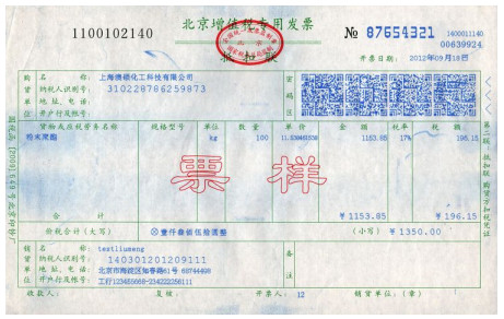
The rapid development and wide application of artificial intelligence is deeply affecting all aspects of human society. Combine artificial intelligence with the accounting industry, use computers to efficiently and automatically process accounting information, and let the accounting industry move towards the intelligent era. This can help people reduce the workload and speed up work efficiency. In recent years, with the rapid development of economy and technology, the use of financial instrument vouchers has exploded, but the processing requirements of financial instrument vouchers have become more and more efficient. Traditional accounting information processing methods, due to the staff's energy and ability, it is often difficult to quickly and accurately handle accounting information. This makes the processing of accounting information lack of timeliness, the degree of utilization of accounting information by enterprises is relatively low, and the demand for intelligent processing of accounting information is constantly pressing. In view of the above problems, this paper uses image processing technology to intelligently identify the content of accounting information to achieve automatic ticket input, improve work efficiency, reduce error rate and reduce labor costs. By simulating the actual 230 invoice images, the results show that the recognition accuracy rate is as high as 98.7%. The results show that the method is effective and has great application value, which is of great significance to the artificial intelligence of accounting information processing.
Citation: Juanjuan Tian, Li Li. Research on artificial intelligence of accounting information processing based on image processing[J]. Mathematical Biosciences and Engineering, 2022, 19(8): 8411-8425. doi: 10.3934/mbe.2022391
The rapid development and wide application of artificial intelligence is deeply affecting all aspects of human society. Combine artificial intelligence with the accounting industry, use computers to efficiently and automatically process accounting information, and let the accounting industry move towards the intelligent era. This can help people reduce the workload and speed up work efficiency. In recent years, with the rapid development of economy and technology, the use of financial instrument vouchers has exploded, but the processing requirements of financial instrument vouchers have become more and more efficient. Traditional accounting information processing methods, due to the staff's energy and ability, it is often difficult to quickly and accurately handle accounting information. This makes the processing of accounting information lack of timeliness, the degree of utilization of accounting information by enterprises is relatively low, and the demand for intelligent processing of accounting information is constantly pressing. In view of the above problems, this paper uses image processing technology to intelligently identify the content of accounting information to achieve automatic ticket input, improve work efficiency, reduce error rate and reduce labor costs. By simulating the actual 230 invoice images, the results show that the recognition accuracy rate is as high as 98.7%. The results show that the method is effective and has great application value, which is of great significance to the artificial intelligence of accounting information processing.

| [1] | J. Wang, Y. Su, Artificial intelligence and accounting model reform, Commun. Finance Account., 22 (2017), 41-43. Available from: https://d.wanfangdata.com.cn/periodical/cktx201722011. |
| [2] | C. Zhang, Analysis of intelligent improvement of accounting information processing, Commun. Finance Account., 34 (2017), 102-105. Available from: https://d.wanfangdata.com.cn/periodical/cktx201734030. |
| [3] | C. Alippi, F. Pessina, M. Roveri, An adaptive system for automatic invoice-documents classification, in IEEE International Conference on Image Processing 2005, 2 (2005), Ⅱ-526. https://doi.org/10.1109/ICIP.2005.1530108 |
| [4] |
Y. Zhang, C. Zhang, S. Yu, J. Yang, Classification of bill image based on frame line detection, J. Nanjing Univ. Sci. Technol. (Nat. Sci.), 31 (2007), 409-413. https://doi.org/10.14177/j.cnki.32-1397n.2007.04.022 doi: 10.14177/j.cnki.32-1397n.2007.04.022

|
| [5] | F. Y. Bu, Q. G. Hu, Y. Wang, A valid frame line removal algorithm for financial document, Comput. Knowl. Technol., 12 (2016), 148-150. Available from: https://d.wanfangdata.com.cn/periodical/dnzsyjs-itrzyksb201623062. |
| [6] | H. Jin, T. Xia, B. Wang, Research on adaptive character segmentation and extraction algorithm, J. Xi'an Univ. Technol., 32 (2016), 399-402+415. Available from: https://xuebao.xaut.edu.cn/__local/2/53/FA/00833B6F761060DF2461CB46334_A0C213DD_120738.pdf?e=.pdf. |
| [7] | W. Sun, A study on XBRL based value chain accounting information processing, in 2017 6th International Conference on Industrial Technology and Management (ICITM), (2017), 171-175. https://doi.org/10.1109/ICITM.2017.7917916 |
| [8] |
W. Cui, L. Ren, Y. Liu, Invoice number recognition algorithm based on numerical structure characteristics, J. Data Acquis. Process., 32 (2017), 119-125. https://doi.org/10.16337/j.1004-9037.2017.01.014 doi: 10.16337/j.1004-9037.2017.01.014
|
| [9] |
H. Ouyang, D. Fan, D. Li, Invoice seal recognition for multi-feature fusion decision making, Comput. Eng. Des., 39 (2018), 2842-2847. https://doi.org/10.16208/j.issn1000-7024.2018.09.026 doi: 10.16208/j.issn1000-7024.2018.09.026
|
| [10] | F. Jiang, H. Chen, L. J. Zhang, FCN-biLSTM based VAT invoice recognition and processing, in Edge Computing - EDGE 2018, (2018), 135-143. https://doi.org/10.1007/978-3-319-94340-4_11 |
| [11] |
J. Shen, L. Han, Design process optimization and profit calculation module development simulation analysis of financial accounting information system based on particle swarm optimization (PSO), Inf. Syst. e-Bus. Manage., 18 (2020), 809-822. https://doi.org/10.1007/s10257-018-00398-0 doi: 10.1007/s10257-018-00398-0
|
| [12] |
Y. Xu, C. Lv, S. Li, P. Xin, S. Ma, H. Zou, et al., Review of development of visual neural computing, Comput. Eng. Appl., 53 (2017), 30-34. https://doi.org/10.3778/j.issn.1002-8331.1709-0474 doi: 10.3778/j.issn.1002-8331.1709-0474
|
| [13] |
Q. Wang, P. Lu, Research on application of artificial intelligence in computer network technology, Int. J. Pattern Recognit. Artif. Intell., 33 (2019), 1959015. https://doi.org/10.1142/S0218001419590158 doi: 10.1142/S0218001419590158
|
| [14] |
X. Liu, Y. Li, Q. Wang, Multi-view hierarchical bidirectional recurrent neural network for depth video sequence based action recognition, Int. J. Pattern Recognit. Artif. Intell., 32 (2018), 1850033. https://doi.org/10.1142/S0218001418500337 doi: 10.1142/S0218001418500337
|
| [15] |
Y. Hou, Q. Wang, Research and improvement of content-based image retrieval framework, Int. J. Pattern Recognit. Artif. Intell., 32 (2018), 1850043. https://doi.org/10.1142/S021800141850043X doi: 10.1142/S021800141850043X
|
| [16] |
Q. Peng, G. Ji, L. Xie, S. Zhang, Application of convolutional neural network in vehicle recognition, J. Front. Comput. Sci. Technol., 12 (2018), 282-291. https://doi.org/10.3778/j.issn.1673-9418.1704055 doi: 10.3778/j.issn.1673-9418.1704055
|
| [17] | X. Zhao, Z. Sun, M. Xia, Vehicle image recognition method based on local learning, J. Zhejiang Univ. Technol., 45 (2017), 439-444. http://xb.qks.zjut.edu.cn/CN/Y2017/V45/I4/439 |
| [18] |
L. Shi, S. Qiang, License plate character recognition based on combined support vector machine. Comput. Eng. Des., 38 (2017), 1619-1623. https://doi.org/10.16208/j.issn1000-7024.2017.06.040 doi: 10.16208/j.issn1000-7024.2017.06.040
|
| [19] |
Q. Gao, Y. Liang, Q. Pan, Y. Chen, H. Zhang, The problem existed in face recognition using SVD and its solution, J. Image Graphics, 11 (2006), 1784-1791. https://doi.org/10.11834/jig.2006012312 doi: 10.11834/jig.2006012312
|
| [20] |
M. Adil, M. K. Khan, M. Jamjoom, A. Farouk, MHADBOR: AI-enabled administrative distance based opportunistic load balancing scheme for an agriculture internet of things network, IEEE Micro, 42 (2022), 41-50. https://doi.org/10.1109/MM.2021.3112264 doi: 10.1109/MM.2021.3112264
|
| [21] |
K. C. Rim, P. K. Kim, H. Ko, K. Bae, T. G. Kwon, Restoration of dimensions for ancient drawing recognition, Electronics, 10 (2021), 2269. https://doi.org/10.3390/electronics10182269 doi: 10.3390/electronics10182269
|
| [22] | A. Xing, X. Tao, R. Peng, Thinking about the accounting industry in the era of artificial intelligence, Account. Learn., 160 (2017), 112+114. Available from: http://www.ckxx.cbpt.cnki.net/WKG/WebPublication/paperDigest.aspx?paperID=9d9ee325-d998-420c-9e18-d24984315f65. |
| [23] | T. Shi, The impact of the rise of artificial intelligence on the future accounting industry, Mod. Bus., 28 (2017), 122-123. https://doi.org/10.14097/j.cnki.5392/2017.28.053 |
| [24] |
M. Ren, Research on the functional transformation of accounting personnel under artificial intelligence, Mod. Bus. Ind., 38 (2017), 68-69. https://doi.org/10.19311/j.cnki.1672-3198.2017.23.030 doi: 10.19311/j.cnki.1672-3198.2017.23.030
|
| [25] | R. Sarkar, S. Halder, S. Malakar, N. Das, S. Basu, M. Nasipuri, Text line extraction from handwritten document pages based on line contour estimation, in 2012 Third International Conference on Computing, Communication and Networking Technologies (ICCCNT'12), (2012), 1-8. https://doi.org/10.1109/ICCCNT.2012.6395873 |
| [26] | W. Wang, An image skew correction method by using directional white run-length, Sci. Technol. Eng., 12 (2012), 5642-5644. Available from: http://www.stae.com.cn/jsygc/article/abstract/121573?st=article_issue. |
| [27] |
J. S. Goldstein, I. S. Reed, L. L. Scharf, A multistage representation of the wiener filter based on orthogonal projections, IEEE Trans. Inf. Theory, 44 (1998), 2943-2959. https://doi.org/10.1109/18.737524 doi: 10.1109/18.737524
|
| [28] |
Y. Yu, J. Li, Denoising research based on wiener filter, J. Luoyang Norm. Univ., 36 (2017), 29-32. https://doi.org/10.16594/j.cnki.41-1302/g4.2017.02.008 doi: 10.16594/j.cnki.41-1302/g4.2017.02.008
|
| [29] |
S. Palanisamy, B. Thangaraju, O. I. Khalaf, Y. Alotaibi, S. Alghamdi, Design and synthesis of multi-mode bandpass filter for wireless applications, Electronics, 10 (2021), 2853. https://doi.org/10.3390/electronics10222853 doi: 10.3390/electronics10222853
|
| [30] |
H. Song, M. Brandt-Pearce, A 2-D discrete-time model of physical impairments in wavelength-division multiplexing systems, J. Lightwave Technol., 30 (2012), 713-726. https://doi.org/10.1109/JLT.2011.2180360 doi: 10.1109/JLT.2011.2180360
|
| [31] | L. Wang, Y. Chen, L. Liu, Research on text image layout segmentation algorithm based on projection contour analysis, Digital Technol. Appl., 3 (2017), 164-165. Available from: http://www.cqvip.com/QK/95792B/20173/671781608.html. |
| [32] |
J. Schmidhuber, Deep learning in neural networks: An overview, Neural Networks, 61 (2015), 85-117. https://doi.org/10.1016/j.neunet.2014.09.003 doi: 10.1016/j.neunet.2014.09.003
|
| [33] | Y. Feng, S. Zeng, Y. Yang, Y. Zhou, B. Pan, Study on the optimization of CNN based on image identification, in 2018 17th International Symposium on Distributed Computing and Applications for Business Engineering and Science (DCABES), (2018), 123-126. https://doi.org/10.1109/DCABES.2018.00041 |
| [34] |
A. Krizhevsky, I. Sutskever, G. E. Hinton, Imagenet classification with deep convolutional neural networks, Commun. ACM, 60 (2017), 84-90. https://doi.org/10.1145/3065386 doi: 10.1145/3065386
|

Figures(2) / Tables(2)

Juanjuan Tian, Li Li. Research on artificial intelligence of accounting information processing based on image processing[J]. Mathematical Biosciences and Engineering, 2022, 19(8): 8411-8425. doi: 10.3934/mbe.2022391


 DownLoad: