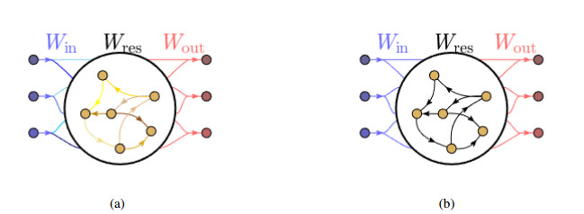
Reservoir computing (RC) is a promising approach for model-free prediction of complex nonlinear dynamical systems. Here, we reveal that the randomness in the parameter configurations of the RC has little influence on its short-term prediction accuracy of chaotic systems. This thus motivates us to articulate a new reservoir structure, called homogeneous reservoir computing (HRC). To further gain the optimal input scaling and spectral radius, we investigate the forecasting ability of the HRC with different parameters and find that there is an ellipse-like optimal region in the parameter space, which is completely beyond the area where the spectral radius is smaller than unity. Surprisingly, we find that this optimal region with better long-term forecasting ability can be accurately reflected by the contours of the $ l_{2} $-norm of the output matrix, which enables us to judge the quality of the parameter selection more directly and efficiently.
Citation: Bolin Zhao. Seeking optimal parameters for achieving a lightweight reservoir computing: A computational endeavor[J]. Electronic Research Archive, 2022, 30(8): 3004-3018. doi: 10.3934/era.2022152
Reservoir computing (RC) is a promising approach for model-free prediction of complex nonlinear dynamical systems. Here, we reveal that the randomness in the parameter configurations of the RC has little influence on its short-term prediction accuracy of chaotic systems. This thus motivates us to articulate a new reservoir structure, called homogeneous reservoir computing (HRC). To further gain the optimal input scaling and spectral radius, we investigate the forecasting ability of the HRC with different parameters and find that there is an ellipse-like optimal region in the parameter space, which is completely beyond the area where the spectral radius is smaller than unity. Surprisingly, we find that this optimal region with better long-term forecasting ability can be accurately reflected by the contours of the $ l_{2} $-norm of the output matrix, which enables us to judge the quality of the parameter selection more directly and efficiently.

| [1] | H. Jaeger, The "echo state" approach to analysing and training recurrent neural networks-with an erratum note, German National Research Center for Information Technology, Bonn, Germany, 148 (2001), 13. |
| [2] |
W. Maass, T. Natschläger, H. Markram, Real-time computing without stable states: A new framework for neural computation based on perturbations, Neural Comput., 14 (2002), 2531–2560. https://doi.org/10.1162/089976602760407955 doi: 10.1162/089976602760407955

|
| [3] |
H. Jaeger, H. Haas, Harnessing nonlinearity: Predicting chaotic systems and saving energy in wireless communication, Science, 304 (2004), 78–80. https://doi.org/10.1126/science.1091277 doi: 10.1126/science.1091277
|
| [4] |
Z. Lu, J. Pathak, B. Hunt, M. Girvan, R. Brockett, E. Ott, Reservoir observers: Model-free inference of unmeasured variables in chaotic systems, Chaos, 27 (2017), 041102. https://doi.org/10.1063/1.4979665 doi: 10.1063/1.4979665
|
| [5] |
J. Pathak, Z. Lu, B. R. Hunt, M. Girvan, E. Ott, Using machine learning to replicate chaotic attractors and calculate lyapunov exponents from data, Chaos, 27 (2017), 121102. https://doi.org/10.1063/1.5010300 doi: 10.1063/1.5010300
|
| [6] |
J. Pathak, B. Hunt, M. Girvan, Z. Lu, E. Ott, Model-free prediction of large spatiotemporally chaotic systems from data: A reservoir computing approach, Phys. Rev. Lett., 120 (2018), 024102. https://doi.org/10.1103/PhysRevLett.120.024102 doi: 10.1103/PhysRevLett.120.024102
|
| [7] |
L. Appeltant, M. C. Soriano, G. Van der Sande, J. Danckaert, S. Massar, J. Dambre, et al., Information processing using a single dynamical node as complex system, Nat. Commun., 2 (2011), 1–6. https://doi.org/10.1038/ncomms1476 doi: 10.1038/ncomms1476
|
| [8] |
A. Rodan, P. Tino, Minimum complexity echo state network, IEEE Trans. Neural Networks, 22 (2010), 131–144. https://doi.org/10.1109/TNN.2010.2089641 doi: 10.1109/TNN.2010.2089641
|
| [9] |
A. Griffith, A. Pomerance, D. J. Gauthier, Forecasting chaotic systems with very low connectivity reservoir computers, Chaos, 29 (2019), 123108. https://doi.org/10.1063/1.5120710 doi: 10.1063/1.5120710
|
| [10] |
M. Buehner, P. Young, A tighter bound for the echo state property, IEEE Trans. Neural Networks, 17 (2006), 820–824. https://doi.org/10.1109/TNN.2006.872357 doi: 10.1109/TNN.2006.872357
|
| [11] | M. Lukosevicius, H. Jaeger, Overview of reservoir recipes, Technical Report, Jacobs University Bremen, 2007. |
| [12] | D. Verstraeten, Reservoir Computing: Computation with Dynamical Systems, Ph.D thesis, Ghent University, 2009. |
| [13] |
I. B. Yildiz, H. Jaeger, S. Kiebel, Re-visiting the echo state property, Neural Networks, 35 (2012), 1–9. https://doi.org/10.1016/j.neunet.2012.07.005 doi: 10.1016/j.neunet.2012.07.005
|
| [14] |
G. Manjunath, H. Jaeger, Echo state property linked to an input: Exploring a fundamental characteristic of recurrent neural networks, Neural Comput., 25 (2013), 671–696. https://doi.org/10.1162/neco_a_00411 doi: 10.1162/neco_a_00411
|
| [15] | S. Basterrech, Empirical analysis of the necessary and sufficient conditions of the echo state property, in 2017 International Joint Conference on Neural Networks, IEEE, (2017), 888–896. https://doi.org/10.1109/IJCNN.2017.7965946 |
| [16] |
J. Jiang, Y. C. Lai, Model-free prediction of spatiotemporal dynamical systems with recurrent neural networks: Role of network spectral radius, Phys. Rev. Res., 1 (2019), 033056. https://doi.org/10.1103/PhysRevResearch.1.033056 doi: 10.1103/PhysRevResearch.1.033056
|
| [17] |
C. G. Langton, Computation at the edge of chaos: Phase transitions and emergent computation, Phys. D, 42 (1990), 12–37. https://doi.org/10.1016/0167-2789(90)90064-V doi: 10.1016/0167-2789(90)90064-V
|
| [18] |
N. Bertschinger, T. Natschläger, Real-time computation at the edge of chaos in recurrent neural networks, Neural Comput., 16 (2004), 1413–1436. https://doi.org/10.1162/089976604323057443 doi: 10.1162/089976604323057443
|
| [19] | N. Bertschinger, T. Natschläger, R. Legenstein, At the edge of chaos: Real-time computations and self-organized criticality in recurrent neural networks, Adv. Neural Inf. Process. Syst., 17 (2004). |
| [20] | B. Schrauwen, D. Verstraeten, J. Van Campenhout, An overview of reservoir computing: theory, applications and implementations, in Proceedings of the 15th European Symposium on Artificial Neural Networks, (2007), 471–482. |
| [21] |
A. Haluszczynski, J. Aumeier, J. Herteux, C. Räth, Reducing network size and improving prediction stability of reservoir computing, Chaos, 30 (2020), 063136. https://doi.org/10.1063/5.0006869 doi: 10.1063/5.0006869
|
| [22] |
Q. Zhu, H. F. Ma, W. Lin, Detecting unstable periodic orbits based only on time series: When adaptive delayed feedback control meets reservoir computing, Chaos, 29 (2019), 093125. https://doi.org/10.1063/1.5120867 doi: 10.1063/1.5120867
|
| [23] |
J. W. Hou, H. F. Ma, D. He, J. Sun, Q. Nie, W. Lin, Harvesting random embedding for high-frequency change-point detection in temporal complex, Natl. Sci. Rev., 2022. https://doi.org/10.1093/nsr/nwab228 doi: 10.1093/nsr/nwab228
|
| [24] |
X. Ying, S. Y. Leng, H. F. Ma, Q. Nie, Y. C. Lai, W. Lin, Continuity scaling: A rigorous framework for detecting and quantifying causality accurately, Research, 2022 (2022), 9870149. https://doi.org/10.34133/2022/9870149 doi: 10.34133/2022/9870149
|


Figures(7) / Tables(2)
Bolin Zhao. Seeking optimal parameters for achieving a lightweight reservoir computing: A computational endeavor[J]. Electronic Research Archive, 2022, 30(8): 3004-3018. doi: 10.3934/era.2022152


 DownLoad: