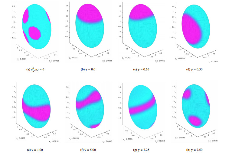
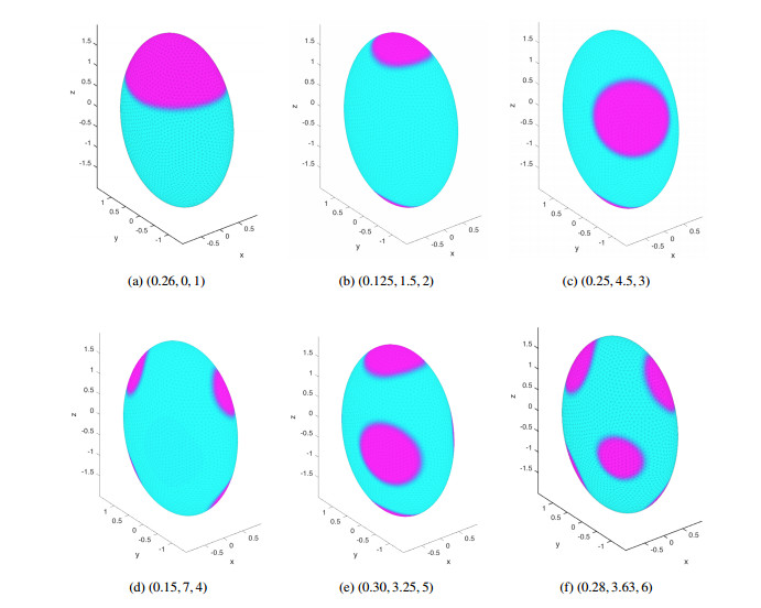
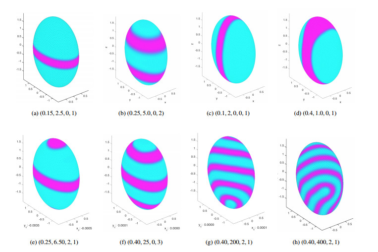
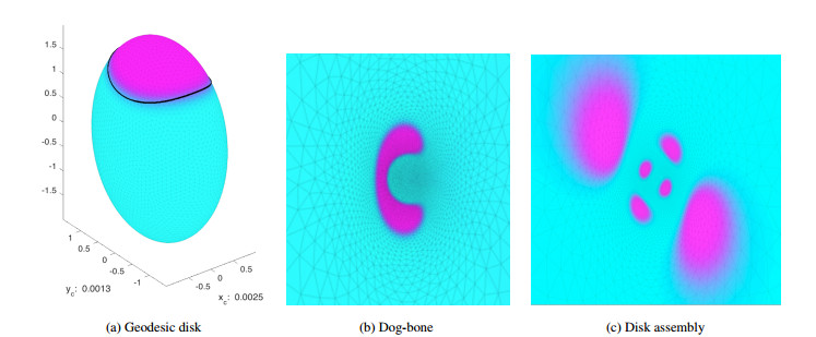
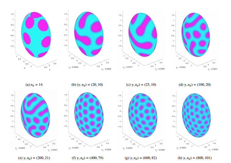
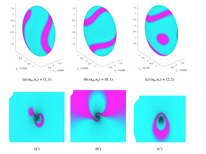
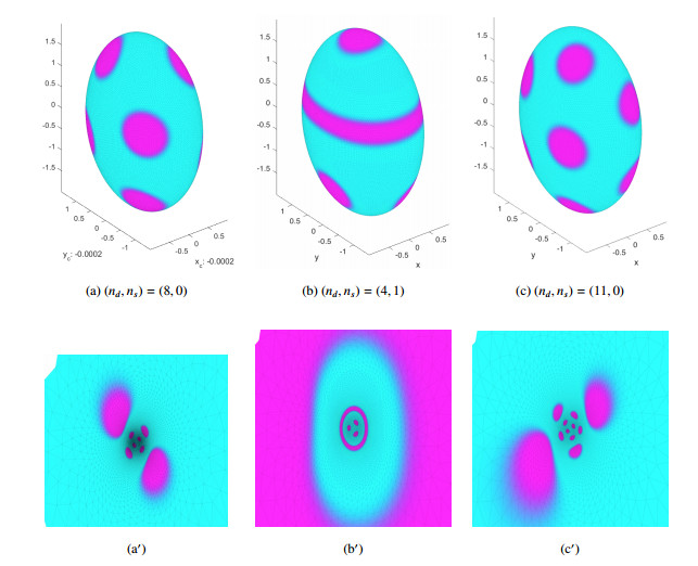
We investigate pattern formation in a two-dimensional manifold using the Otha-Kawasaki model for micro-phase separation of diblock copolymers. In this model, the total energy includes a short-range and a long-range term. The short-range term is a Landau-type free energy that is common in phase separation problems and favors large domains with minimum perimeter. The inhibitory long-range interaction term is the Otha-Kawasaki functional derived from the theory of diblock copolymers and favors small domains. The balance of these terms leads to equilibrium states that exhibit a variety of patterns, including disk-like droplets, droplet assemblies, elongated droplets, dog-bone shaped droplets, stripes, annular rings, wriggled stripes and combinations thereof. For problems where analytical results are known, we compare our numerical results and find good agreement. Where analytical results are not available, our numerical methods allow us to explore the solution space revealing new stable patterns. We focus on the triaxial ellipsoid, but our methods are general and can be applied to higher genus surfaces and surfaces with boundaries.
Citation: Frank Baginski, Jiajun Lu. Numerical investigations of pattern formation in binary systems with inhibitory long-range interaction[J]. Electronic Research Archive, 2022, 30(5): 1606-1631. doi: 10.3934/era.2022081
We investigate pattern formation in a two-dimensional manifold using the Otha-Kawasaki model for micro-phase separation of diblock copolymers. In this model, the total energy includes a short-range and a long-range term. The short-range term is a Landau-type free energy that is common in phase separation problems and favors large domains with minimum perimeter. The inhibitory long-range interaction term is the Otha-Kawasaki functional derived from the theory of diblock copolymers and favors small domains. The balance of these terms leads to equilibrium states that exhibit a variety of patterns, including disk-like droplets, droplet assemblies, elongated droplets, dog-bone shaped droplets, stripes, annular rings, wriggled stripes and combinations thereof. For problems where analytical results are known, we compare our numerical results and find good agreement. Where analytical results are not available, our numerical methods allow us to explore the solution space revealing new stable patterns. We focus on the triaxial ellipsoid, but our methods are general and can be applied to higher genus surfaces and surfaces with boundaries.

| [1] |
K. Kawasaki, T. Ohta, M. Kohrogui, Equilibrium morphology of block copolymer melts. 2, Macromolecules, 21 (1988), 2972–2980. https://doi.org/10.1021/ma00188a014 doi: 10.1021/ma00188a014

|
| [2] |
T. Ohta, K. Kawasaki, Equilibrium morphology of block copolymer melts, Macromolecules, 19 (1986), 2621–2632. https://doi.org/10.1021/ma00164a028 doi: 10.1021/ma00164a028
|
| [3] |
R. Choksi, X. Ren, On the derivation of a density functional theory for microphase separation of diblock copolymers, J. Stat. Phys., 113 (2003), 151–176. https://doi.org/10.1023/A:1025722804873 doi: 10.1023/A:1025722804873
|
| [4] | H. Kielhofer, Pattern Formation of the Stationary Cahn-Hilliard Model, Chaotic Model. Simul., 1 (2011), 29–38. |
| [5] | Y. Hu, Disc Assemblies and Spike Assemblies in Inhibitory Systems, PhD thesis, Department of Mathematics, George Washington University, 2016. |
| [6] |
X. Ren, J. Wei, Many droplet pattern in the cylindrical phase of diblock copolymer morphology, Rev. Math. Phys., 19 (2007), 879–921. https://doi.org/10.1142/S0129055X07003139 doi: 10.1142/S0129055X07003139
|
| [7] |
X. Ren, J. Wei, Oval shaped droplet solutions in the saturation process of some pattern formation problems, SIAM J. Appl. Math., 70 (2009), 1120–1138. https://doi.org/10.1137/080742361 doi: 10.1137/080742361
|
| [8] |
X. Ren, J. Wei, Wriggled lamellar solutions and their stability in the diblock copolymer problem, SIAM J. Math. Anal., 37 (2005), 455–489. https://doi.org/10.1137/S0036141003433589 doi: 10.1137/S0036141003433589
|
| [9] |
C. B. Muratov, Theory of domain patterns in systems with long-range interactions of coulomb type, Phys. Rev. E (3), 66 (2002), 066108. https://doi.org/10.1103/PhysRevE.66.066108 doi: 10.1103/PhysRevE.66.066108
|
| [10] |
X. Chen, Y. Oshita, Periodicity and uniqueness of global minimizers of an energy functional containing a long-range interaction, SIAM J. Math. Anal., 37 (2005), 1299–1332. https://doi.org/10.1137/S0036141004441155 doi: 10.1137/S0036141004441155
|
| [11] |
X. Ren, J. Wei, On energy minimzers of the diblock copolymer problem, Interface. Free Bound., 5 (2003), 193–238. https://doi.org/10.4171/IFB/78 doi: 10.4171/IFB/78
|
| [12] |
P. Sternberg, I. Topaloglu, On the global minimizers of a nonlocal isoperimetric problem in two dimensions, Interface. Free Bound., 13 (2011), 155–169. https://doi.org/10.4171/IFB/252 doi: 10.4171/IFB/252
|
| [13] |
I. Topaloglu, On a nonlocal isoperimetric problem on the two-sphere, Commun. Pure Appl. Anal., 12 (2013), 597–620. https://doi.org/10.3934/cpaa.2013.12.597 doi: 10.3934/cpaa.2013.12.597
|
| [14] |
D. Crowdy, M. Cloke, Analytical solutions for distributed multipolar vortex equilibria on a sphere, Phys. Fluids, 15 (2003), 22–34. https://doi.org/10.1063/1.1521727 doi: 10.1063/1.1521727
|
| [15] |
J. Lu, F. Baginski, X. Ren, Equilibrium configurations of boundary droplets in a self-organizing inhibitory system, SIAM J. Appl. Dyn. Syst., 17 (2018), 1353–1376. https://doi.org/10.1137/17M113856X doi: 10.1137/17M113856X
|
| [16] |
S. Gillmor, J. Lee, X. Ren, The role of Gauss curvature in a membrane phase separation problem, Physica D, 240 (2011), 1913–1927. https://doi.org/10.1016/j.physd.2011.09.002 doi: 10.1016/j.physd.2011.09.002
|
| [17] | T. Aubin, Nonlinear Analysis on Manifolds. Monge-Amperé Equations, Springer-Verlag, New York, 1980. |
| [18] | S. Larsson, V. Thomée, Partial Differential Equations with Numerical Methods, Springer-Verlag, 2003. |
| [19] |
P. O. Persson, G. Strang, A simple mesh generator in MATLAB, SIAM Rev., 46 (2004), 329–345. https://doi.org/10.1137/S0036144503429121 doi: 10.1137/S0036144503429121
|
| [20] |
F. Baginski, R. Croce, S. Gillmor, R. Krause, Numerical investigations of the role of curvature in strong segregation problems on a given surface, Appl. Math. Comput., 227 (2014), 399–411. https://doi.org/10.1016/j.amc.2013.11.008 doi: 10.1016/j.amc.2013.11.008
|
Figures(11) / Tables(6)
Frank Baginski, Jiajun Lu. Numerical investigations of pattern formation in binary systems with inhibitory long-range interaction[J]. Electronic Research Archive, 2022, 30(5): 1606-1631. doi: 10.3934/era.2022081


 DownLoad: