The interpretation of dissipation tests from cone penetration tests (CPTU) in silt is often considered challenging due to the occurrence of an unknown degree of partial consolidation during penetration which may influence the results significantly. The main objective of the present study is to investigate the influence of penetration rate and hence partial consolidation in silt deposits on the interpretation of consolidation parameters. Rate dependency studies have been carried out so as to give recommendations on how to establish design consolidation parameters in silts and consider the effect of partial consolidation on the development of design parameters. A comprehensive field and laboratory research program has been conducted on a silt deposit in Halsen-Stj?rdal, Norway. Alongside performing various rate penetration CPTU tests with rates varying between 0.5 mm/s and 200 mm/s, dissipation tests were executed to analyze the consolidation behaviour of the soil deposit. Furthermore, a series of soil samples have been taken at the site to carry out high quality laboratory tests. Correction methods developed for non-standard dissipation tests could be successfully applied to the silt deposit indicating partial consolidation. The results revealed an underestimation of the coefficient of consolidation if partial consolidation is neglected in the analysis, emphasizing the importance of considering the drainage conditions at a silt site thoroughly. To study the drainage conditions of a soil deposit a recently proposed approach has been applied introducing a normalized penetration rate to differentiate between drained and undrained behaviour during penetration. It is suggested that a normalized penetration rate of less than 0.1–0.2 indicate drained behaviour while a normalized penetration rate above 40–50 indicate undrained behaviour. Finally, available dissipation test data from a Norwegian Geo-Test Site (NGTS) in Halden, Norway have been used to successfully verify the recommendations made for silts.
Citation: Annika Bihs, Mike Long, Steinar Nordal, Priscilla Paniagua. Consolidation parameters in silts from varied rate CPTU tests[J]. AIMS Geosciences, 2021, 7(4): 637-668. doi: 10.3934/geosci.2021039
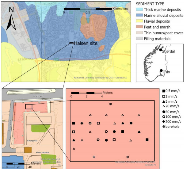
The interpretation of dissipation tests from cone penetration tests (CPTU) in silt is often considered challenging due to the occurrence of an unknown degree of partial consolidation during penetration which may influence the results significantly. The main objective of the present study is to investigate the influence of penetration rate and hence partial consolidation in silt deposits on the interpretation of consolidation parameters. Rate dependency studies have been carried out so as to give recommendations on how to establish design consolidation parameters in silts and consider the effect of partial consolidation on the development of design parameters. A comprehensive field and laboratory research program has been conducted on a silt deposit in Halsen-Stj?rdal, Norway. Alongside performing various rate penetration CPTU tests with rates varying between 0.5 mm/s and 200 mm/s, dissipation tests were executed to analyze the consolidation behaviour of the soil deposit. Furthermore, a series of soil samples have been taken at the site to carry out high quality laboratory tests. Correction methods developed for non-standard dissipation tests could be successfully applied to the silt deposit indicating partial consolidation. The results revealed an underestimation of the coefficient of consolidation if partial consolidation is neglected in the analysis, emphasizing the importance of considering the drainage conditions at a silt site thoroughly. To study the drainage conditions of a soil deposit a recently proposed approach has been applied introducing a normalized penetration rate to differentiate between drained and undrained behaviour during penetration. It is suggested that a normalized penetration rate of less than 0.1–0.2 indicate drained behaviour while a normalized penetration rate above 40–50 indicate undrained behaviour. Finally, available dissipation test data from a Norwegian Geo-Test Site (NGTS) in Halden, Norway have been used to successfully verify the recommendations made for silts.

| [1] | Blaker Ø (2020) Characterization of a Natural Clayey Silt and the Effects of Sample Disturbance on Soil Behavior and Engineering Properties. |
| [2] | Silva MF, Bolton MD (2005) Interpretation of Centrifuge Piezocone Tests in Dilatant, Low Plasticity Silts. Int Conf Probl Soils, 1277-1284. |
| [3] |
Schneider JA, Lehane BM, Schnaid F (2007) Velocity Effects on Piezocone Measurements in Normally and Overconsolidated Clays. Int J Phys Modell Geotech 7: 23-34. doi: 10.1680/ijpmg.2007.070202

|
| [4] | Mahmoodzadeh H, Randolph MF (2014) Penetrometer Testing: Effect of Partial Consolidation on Subsequent Dissipation Response. J Geotech Geoenviron Eng 140. |
| [5] | Schnaid F, Nierwinski HP, Odebrecht E (2020) Classification and State-Parameter Assessment of Granular Soils Using the Seismic Cone. J Geotech Geoenviron Eng 146. |
| [6] | Viana da Fonseca A, Molina-Gomez F, Ferreira C, et al. (2021) An integrated interpretation of SCPTu for liquefaction assessment in intermediate alluvial deposits in Portugal. 6th Int Conf Geotech Geopgys Site Charact. |
| [7] |
Holmsgaard R, Nielsen BN, Ibsen LB (2016) Interpretation of Cone Penetration Testing in Silty Soils Conducted under Partially Drained Conditions. J Geotech Geoenviron Eng 142: 04015064. doi: 10.1061/(ASCE)GT.1943-5606.0001386
|
| [8] |
Blaker Ø, Carroll R, Paniagua P, et al. (2019) Halden Research Site: Geotechnical Characterization of a Post Glacial Silt. AIMS Geosci 5: 184-234. doi: 10.3934/geosci.2019.2.184
|
| [9] | Krage CP, Albin B, DeJong JT, et al. (2016) The Influence of In-situ Effective Stress on Sample Quality for Intermediate Soils. Geotech Geophys Site Charact 5, 565-570. |
| [10] | Bihs A, Long M, Nordal S (2021) Evaluation of Soil Strength from Variable Rate CPTU Tests in Silt. Geotech Test J. |
| [11] |
Sully JP, Robertson PK, Campanella RG, et al. (1999) An Approach to Evaluation of Field CPTU Dissipation Data in Overconsolidated Fine-Grained Soils. Can Geotech J 36: 369-381. doi: 10.1139/t98-105
|
| [12] |
Burns SE, Mayne PW (1998) Monotonic and Dilatory Pore-pressure Decay during Piezocone Tests in Clay. Can Geotech J 35: 1063-1073. doi: 10.1139/t98-062
|
| [13] |
Chai JC, Sheng D, Carter JP, et al. (2012) Coefficient of Consolidation from Non-standard Piezocone Dissipation Curves. Comput Geotech 41: 13-22. doi: 10.1016/j.compgeo.2011.11.005
|
| [14] |
Teh CI, Houlsby GT (1991) An Analytical Study on the Cone Penetration Test in Clay. Géotechnique 41: 17-34. doi: 10.1680/geot.1991.41.1.17
|
| [15] |
DeJong JT, Randolph M (2012) Influence of Partial Consolidation during Cone Penetration on Estimated Soil Behavior Type and Pore Pressure Dissipation Measurements. J Geotech Geoenviron Eng 138: 777-788. doi: 10.1061/(ASCE)GT.1943-5606.0000646
|
| [16] |
Schnaid F, Dienstmann G, Odebrecht E, et al. (2020) A Simplified Approach to Normalisation of Piezocone Penetration Rate Effects. Géotechnique 70: 630-635. doi: 10.1680/jgeot.18.T.033
|
| [17] | Sveian H (1995) Sandsletten blir til: Stjørdal fra Fjordbunn til Strandsted (in Norwegian). Trondheim: Norges Geologiske Undersøkelse (NGU). |
| [18] | Sandven R (2003) Geotechnical Properties of a Natural Silt Deposit obtained from Field and Laboratory Tests. Int Workshop Charact Eng Prop Nat Soils, 1121-1148. |
| [19] | NGU (2021) Quaternary map Norway. Geological Survey of Norway (NGU). Available from: http://geo.ngu.no/kart/losmasse_mobil/. |
| [20] |
Bihs A, Long M, Nordal S (2020) Geotechnical Characterization of Halsen-Stjørdal Silt, Norway. AIMS Geosci 6: 355-377. doi: 10.3934/geosci.2020020
|
| [21] | Lunne T, Berre T, Strandvik S (1997) Sample Disturbance Effects in Soft Low Plastic Norwegian Clay. Recent Developments in Soil and Pavement Mechanics, Rio de Janeiro, Brazil: Balkema, 81-102. |
| [22] | Andresen A, Kolstad P (1979) The NGI 54 mm Sampler for Undisturbed Sampling of Clays and Representative Sampling of Coarse Materials, International Symposium on Soil Sampling. Singapore, 13-21. |
| [23] |
DeJong JT, Krage CP, Albin BM, et al. (2018) Work-Based Framework for Sample Quality Evaluation of Low Plasticity Soils. J Geotech Geoenviron Eng 144: 04018074. doi: 10.1061/(ASCE)GT.1943-5606.0001941
|
| [24] | NGF (2011) Melding 2: Veiledning for Symboler og Definisjoner i Geoteknikk—Identifisering og Klassifisering av Jord (in Norwegian). Oslo, Norway: Norwegian Geotechnical Society. Available from: www.ngf.no. |
| [25] | Sandbaekken G, Berre T, Lacasse S (1986) Oedometer Testing at the Norwegian Geotechnical Institute. ASTM Spe Tech Publ, 329-353. |
| [26] |
Long M, Gudjonsson G, Donohue S, et al. (2010) Engineering Characterisation of Norwegian Glaciomarine Silt. Eng Geol 110: 51-65. doi: 10.1016/j.enggeo.2009.11.002
|
| [27] |
Boone SJ (2010) A Critical Reappraisal of "Preconsolidation Pressure" Interpretations using the Oedometer Test. Can Geotech J 47: 281-296. doi: 10.1139/T09-093
|
| [28] |
Becker DE, Crooks JHA, Been K, et al. (1987) Work as a Criterion for Determining In Situ and Yield Stresses in Clays. Can Geotech J 24: 549-564. doi: 10.1139/t87-070
|
| [29] | Janbu N (1963) Soil Compressibility as Determined by Oedometer and Triaxial Tests. ECSMFE. Wiesbaden, Germany, 19-25. |
| [30] |
Berre T (1982) Triaxial Testing at the Norwegian Geotechnical Institute. Geotech Test J 5: 3-17. doi: 10.1520/GTJ10794J
|
| [31] |
Brandon TL, Rose AT, Duncan JM (2006) Drained and Undrained Strength Interpretation for Low-Plasticity Silts. J Geotech Geoenviron Eng 132: 250-257. doi: 10.1061/(ASCE)1090-0241(2006)132:2(250)
|
| [32] | Krage CP, Broussard NS, Dejong JT (2014) Estimating Rigidity Index based on CPT Measurements. Int Symp Cone Penetration Test, 727-735. |
| [33] |
Schnaid F, Sills GC, Soares JM, et al. (1997) Predictions of the Coefficient of Consolidation from Piezocone Tests. Can Geotech J 34: 315-327. doi: 10.1139/t96-112
|
| [34] | Keaveny JM, Mitchell J (1986) Strength of Fine-grained Soils using the Piezocone. Use In-Situ Tests Geotech Eng, 668-685. |
| [35] | Kulhawy FH, Mayne PW (1990) Manual on Estimating Soil Properties for Foundation Design. Electr Power Res Inst, 1-308. |
| [36] | Mayne PW (2001) Stress-strain-strength-flow Parameters from Enhanced In-situ Tests. Int Conf In-Situ Meas Soil Prop Case Hist, 27-48. |
| [37] | Agaiby SS, Mayne PW (2018) Evaluating Undrained Rigidity Index of Clays from Piezocone date, Cone Penetration Testing (CPT18), Delft, The Netherlands: CRC Press. |
| [38] | Carroll R, Paniagua P (2018) Variable Rate of Penetration and Dissipation Test Results in a Natural Silty Soil. Cone Penetration Testing (CPT18). Delft University of Technology, The Netherlands: CRC Press/Balkema Taylor & Grancis Group, 205-212. |
| [39] | Suzuki Y, Lehane B, Fourie A (2013) Effect of Penetration Rate on Piezocone Parameters in Two Silty Deposits. Fourth Int Conf Site Charact 1: 809-815. |
| [40] | Garcia Martinez MF, Tonni L, Gottardi G, et al. (2016) Influence of Penetration Rate on CPTU Measurements in Saturated Silty Soils. Fifth Int Conf Geotech Geophys Site Charact, 473-478. |
| [41] | Garcia Martinez MF, Tonni L, Gottard G, et al. (2018) Analysis of CPTU Data for the Geotechnical Characterization of Intermediate Sediments, Cone Penetration Testing 2018, Delft, The Netherlands: CRC Press, 281-287. |
| [42] |
Tonni L, Gottard G (2019) Assessing Compressibility Characteristics of Silty Soils from CPTU: Lessons Learnt from the Treporti Test Site, Venetian Lagoon (Italy). AIMS Geosci 5: 117-144. doi: 10.3934/geosci.2019.2.117
|
| [43] | International Organization for Standardization (2012) Geotechnical Investigation and Testing— Field Testing. Part I: Electrical Cone and Piezocone Penetration Test. Geneva, Switzerland, 1-46. |
| [44] | Chai JC, Carter JP, Miura N, et al. (2004) Coefficient of Consolidation from Piezocone Dissipation Tests. Int Symp Lowland Technol, 1-6. |
| [45] | Campanella RG, Robertson PK, Gillespie D (1981) In-situ Testing in Saturated Silt (Drained or Undrained?). 34th Can Geotech Conf, 521-535. |
| [46] |
Wroth CP (1984) The Interpretation of In Situ Soil Tests. Géotechnique 34: 449-489. doi: 10.1680/geot.1984.34.4.449
|
| [47] | Mayne PW, Bachus RC (1988) Profiling OCR in Clays by Piezocone Soundings. Orlando: Balkema, Rotterdam, 857-864. |
| [48] |
Chow SH, O'Loughlin CD, Zhou Z, et al. (2020) Penetrometer Testing in a Calcareous Silt to Explore Changes in Soil Strength. Géotechnique 70: 1160-1173. doi: 10.1680/jgeot.19.P.069
|
| [49] | Lunne T, Robertson PK, Powell JJM (1997) Cone Penetration Testing in Geotechnical Practice, London: Blackie Academic & Professional. |
| [50] | DeJong JT, Jaeger R, Boulanger R, et al. (2013) Variable Penetration Rate Cone Testing for Characterization of Intermediate Soils. Geotech Geophys Site Charact 4, 25-42. |
| [51] |
Robertson PK, Sully JP, Woeller DJ, et al. (1992) Estimating Coefficient of Consolidation from Piezocone Tests. Can Geotech J 29: 539-550. doi: 10.1139/t92-061
|
| [52] | Paniagua P, Carroll R, L'Heureux JS, et al. (2016) Monotonic and Dilatory Excess Pore Water Dissipations in Silt Following CPTU at Variable Penetration Rate. Fifth Int Conf Geotech Geophys Site Charact, 509-514. |
| [53] | Krage CP, Dejong JT, Degroot D, et al. (2015) Applicability of Clay-Based Sample Disturbance Criteria to Intermediate Soils. Int Conf Earthquake Geotech Eng. |
| [54] |
Mahmoodzadeh H, Randolph MF, Wang D (2014) Numerical Simulation of Piezocone Dissipation Test in Clays. Géotechnique 64: 657-666. doi: 10.1680/geot.14.P.011
|
| [55] | Randolph MF (2016) New Tools and Directions in Offshore Site Investigation. Aust Geomech J 51: 81-92. |
| [56] |
Parez L, Fauriel R (1988) Le Piezocone Améliorations Apportées à la Reconnaissance des Sols. Rev Fr de Géotechnique 44: 13-27. doi: 10.1051/geotech/1988044013
|
| [57] | Robertson PK (2010) Soil Behaviour Type from the CPT: an Update. Int Symp Cone Penetration Test. |
| [58] | Finnie IMS, Randolph M (1994) Punch-Through and Liquefaction Induced Failure of Shallow Foundations on Calcerous Sediments. Seventh Int Conf Behav Offshore Struct, 217-230. |
| [59] |
House AR, Oliveira JRMS, Randolph MF (2001) Evaluating the Coefficient of Consolidation Using Penetration Tests. Int J Phys Modell Geotech 1: 17-26. doi: 10.1680/ijpmg.2001.010302
|
| [60] |
Chung SF, Randolph MF, Schneider JA (2006) Effect of Penetration Rate on Penetrometer Resistance in Clay. J Geotech Geoenviron Eng 132: 1188-1196. doi: 10.1061/(ASCE)1090-0241(2006)132:9(1188)
|
| [61] | Senneset K, Sandven R, Lunne T, et al. (1988) Piezocone Tests in Silty Soils. First Int Symp Penetration Test, 955-966. |


Figures(23) / Tables(1)

Annika Bihs, Mike Long, Steinar Nordal, Priscilla Paniagua. Consolidation parameters in silts from varied rate CPTU tests[J]. AIMS Geosciences, 2021, 7(4): 637-668. doi: 10.3934/geosci.2021039


 DownLoad: