
Citation: Amy Mizen, Richard Fry, Daniel Grinnell, Sarah E. Rodgers. Quantifying the Error Associated with Alternative GIS-based Techniques to Measure Access to Health Care Services[J]. AIMS Public Health, 2015, 2(4): 746-761. doi: 10.3934/publichealth.2015.4.746
[1] | Shuguang Li, Mingsong Li, Muhammad Ijaz Khan . Algorithms for two-agent unbounded serial-batch scheduling with makespan and maximum lateness objectives. Networks and Heterogeneous Media, 2023, 18(4): 1678-1691. doi: 10.3934/nhm.2023073 |
[2] | Dieter Armbruster, Michael Herty, Xinping Wang, Lindu Zhao . Integrating release and dispatch policies in production models. Networks and Heterogeneous Media, 2015, 10(3): 511-526. doi: 10.3934/nhm.2015.10.511 |
[3] | Qi Luo, Ryan Weightman, Sean T. McQuade, Mateo Díaz, Emmanuel Trélat, William Barbour, Dan Work, Samitha Samaranayake, Benedetto Piccoli . Optimization of vaccination for COVID-19 in the midst of a pandemic. Networks and Heterogeneous Media, 2022, 17(3): 443-466. doi: 10.3934/nhm.2022016 |
[4] | Mostafa Zahri, Inayat khan, Rahat Zarin, Amir khan, Rukhsar Ikram . A machine learning solutions approach of a time-delayed stochastic $ \tilde{S}\tilde{E}\tilde{I}\tilde{R}\tilde{V} $ model. Networks and Heterogeneous Media, 2025, 20(2): 701-731. doi: 10.3934/nhm.2025030 |
[5] | Lichen Sun, Xu Fang, Hongze Yang, Wenbo Zhong, Bo Li . Visualizing thematic evolution in intelligent cockpit emotion perception: A Bibliometric analysis with CiteSpace and VOSviewer. Networks and Heterogeneous Media, 2025, 20(2): 428-459. doi: 10.3934/nhm.2025020 |
[6] | Vincent Renault, Michèle Thieullen, Emmanuel Trélat . Optimal control of infinite-dimensional piecewise deterministic Markov processes and application to the control of neuronal dynamics via Optogenetics. Networks and Heterogeneous Media, 2017, 12(3): 417-459. doi: 10.3934/nhm.2017019 |
[7] | Don A. Jones, Hal L. Smith, Horst R. Thieme . Spread of viral infection of immobilized bacteria. Networks and Heterogeneous Media, 2013, 8(1): 327-342. doi: 10.3934/nhm.2013.8.327 |
[8] | Giuseppe Buttazzo, Filippo Santambrogio . Asymptotical compliance optimization for connected networks. Networks and Heterogeneous Media, 2007, 2(4): 761-777. doi: 10.3934/nhm.2007.2.761 |
[9] | Cristian Barbarosie, Anca-Maria Toader . Optimization of bodies with locally periodic microstructure by varying the periodicity pattern. Networks and Heterogeneous Media, 2014, 9(3): 433-451. doi: 10.3934/nhm.2014.9.433 |
[10] | Al-hassem Nayam . Asymptotics of an optimal compliance-network problem. Networks and Heterogeneous Media, 2013, 8(2): 573-589. doi: 10.3934/nhm.2013.8.573 |
Parallel machine scheduling has received extensive attention since 1950, given the wide diversity of real-world systems it represents. A variety of criteria has been considered. Among the most studied criteria are makespan (maximum completion time) and total completion time, which can measure the effective utilization of the machines. A second set of criteria are related to meeting due dates and thus considering the system's customers. If the criteria are not specified, we can consider two types of general objective functions: min-sum and min-max.
In real production, decision makers may need to consider a number of criteria simultaneously before arriving at a decision. However, it is often the case that different criteria are in conflict. A solution which is optimal with respect to a given criterion might be a poor candidate for some other criterion. Thus, in the last two decades, multicriteria optimization approaches and techniques have been increasingly applied to provide solutions where the criteria are balanced in an acceptable and profitable way [1,2].
An important subclass in multicriteria optimization is bicriteria optimization where only two criteria, say $ {{\gamma }^{1}} $ and $ {{\gamma }^{2}} $, are considered. There are four popular approaches in the literature: (a) Positive combination optimization: find a schedule to minimize the positive linear combination of $ {{\gamma }^{1}} $ and $ {{\gamma }^{2}} $. (b) Constrained optimization: find a schedule to minimize $ {{\gamma }^{2}} $ under an upper bound on $ {{\gamma }^{1}} $. (c) Pareto optimization (also called simultaneous optimization): find all Pareto-optimal solutions for $ {{\gamma }^{1}} $ and $ {{\gamma }^{2}} $. A feasible schedule $ \sigma $ is (strict) Pareto-optimal for $ {{\gamma }^{1}} $ and $ {{\gamma }^{2}} $ if there is no feasible schedule $ {\sigma }' $ such that $ {{\gamma }^{1}}({\sigma }')\le {{\gamma }^{1}}(\sigma) $ and $ {{\gamma }^{2}}({\sigma }')\le {{\gamma }^{2}}(\sigma) $, where at least one of the inequalities is strict. The objective vector $ ({{\gamma }^{1}}(\sigma), {{\gamma }^{2}}(\sigma)) $ of a Pareto-optimal schedule $ \sigma $ is called a Pareto-optimal point [1]. A feasible schedule $ \sigma $ is weak Pareto-optimal for $ {{\gamma }^{1}} $ and $ {{\gamma }^{2}} $ if there is no feasible schedule $ {\sigma }' $ such that $ {{\gamma }^{1}}({\sigma }') < {{\gamma }^{1}}(\sigma) $ and $ {{\gamma }^{2}}({\sigma }') < {{\gamma }^{2}}(\sigma) $. (d) Hierarchical optimization (also called lexicographical optimization): find a schedule to minimize $ {{\gamma }^{2}} $ among the set of optimal schedules minimizing $ {{\gamma }^{1}} $. In hierarchical bicriteria scheduling problems, the two criteria have different levels of importance thus they are optimized in a lexicographic fashion. Such problems appear naturally in situations where there are several optimal solutions with respect to a specific objective and the decision maker needs to select from among these solutions the one with the best second objective.
In this paper, we consider the bicriteria problem of scheduling equal-processing-time jobs with release dates non-preemptively on identical machines. We apply a Pareto optimization approach to minimize the total completion time (and makespan) and maximum cost simultaneously, and we apply a hierarchical optimization approach to minimize two general min-max criteria hierarchically.
Formally speaking, we are given a set of $ n $ jobs, $ \mathcal{J} = \{{{J}_{1}}, {{J}_{2}}, \ldots, {{J}_{n}}\} $, to be processed on $ m $ identical machines. The machines run in parallel and each machine can process at most one job at a time. All jobs have the same processing time $ p > 0 $. Each job, $ {{J}_{j}}\in \mathcal{J} $, has a release date $ {{r}_{j}}\ge 0 $ before which it cannot be processed, as well as two cost functions $ {{f}_{j}}(t) $ and $ {{g}_{j}}(t) $ which denote the costs incurred if the job is completed at time $ t $. We assume that all $ {{f}_{j}} $ and $ {{g}_{j}} $ are regular, i.e., $ {{f}_{j}} $ and $ {{g}_{j}} $ are non-decreasing in the job completion times [3].
A schedule assigns each job $ {{J}_{j}} $ to exactly one machine and specifies its completion time $ {{C}_{j}} $ on the machine. Given a schedule $ \sigma $, let $ {{f}_{j}}({{C}_{j}}(\sigma)) $ and $ {{g}_{j}}({{C}_{j}}(\sigma)) $ be two scheduling costs of $ {{J}_{j}} $. Then $ {{f}_{\max }}(\sigma) = {{\max }_{j}}{{f}_{j}}({{C}_{j}}(\sigma)) $ and $ {{g}_{\max }}(\sigma) = {{\max }_{j}}{{g}_{j}}({{C}_{j}}(\sigma)) $ are two maximum costs of $ \sigma $. Two important special cases of maximum cost are the makespan $ {{C}_{\max }}(\sigma) = {{\max }_{j}}\{{{C}_{j}}(\sigma)\} $ and the maximum lateness $ {{L}_{\max }}(\sigma) = {{\max }_{j}}\{{{C}_{j}}(\sigma)-{{d}_{j}}\} $, where $ d_j $ denotes the due date of job $ J_j $. We omit the argument $ \sigma $ when it is clear to which schedule we are referring.
The first bicriteria problem we consider is to determine Pareto-optimal schedules which simultaneously minimize the total completion time $ \sum\nolimits_{j = 1}^{n}{{{C}_{j}}} $ (and makespan $ {{C}_{\max }} $) and maximum cost $ {{f}_{\max }} $. Following the notation schemes of [1,2,3], it can be denoted by $ P|{{r}_{j}}, {{p}_{j}} = p|(\sum\nolimits_{j = 1}^{n}{{{C}_{j}}}, {{f}_{\max }}) $ (and $ P|{{r}_{j}}, {{p}_{j}} = p|({{C}_{\max }}, {{f}_{\max }}) $).
The second bicriteria problem we consider is to determine a lexicographical optimal schedule such that the secondary criterion $ {{g}_{\max }} $ is minimized under the constraint that the primary criterion $ {{f}_{\max }} $ is minimized. Following the notation schemes of [1,2,3], it can be denoted by $ P|{{r}_{j}}, {{p}_{j}} = p|Lex({{f}_{\max }}, {{g}_{\max }}) $, where the criterion mentioned first in the argument of $ Lex $ is the more important one.
For parallel machine scheduling that considers multiple criteria, please refer to [4,5,6] for the surveys. Examples of Pareto optimization and hierarchical optimization scheduling on parallel machines can be found in [7,8,9,10,11] and [12,13,14], respectively.
Bruno et al. [15] proved that problem $ P\vert \vert Lex(\sum\nolimits_{j = 1}^{n}{{{C}_{j}}}, {{C}_{\max }}) $ (the jobs have unequal processing times and equal release dates) is NP-hard. Gupta et al. [16] further gave a complexity result: they showed that $ P\vert \vert Lex(\sum\nolimits_{j = 1}^{n}{{{C}_{j}}}, {{C}_{\max }}) $ is strongly NP-hard. Hence, Pareto optimization problem $ P\vert \vert (\sum\nolimits_{j = 1}^{n}{{{C}_{j}}}, {{f}_{\max }}) $ is also strongly NP-hard. Since the single criterion problem $ P\vert \vert {{C}_{\max }} $ is strongly NP-hard [17], the lexicographical optimization problem $ P\vert \vert Lex({{f}_{\max }}, {{g}_{\max }}) $ is strongly NP-hard, too. Also, problem $ 1|{{r}_{j}}|(\sum\nolimits_{j = 1}^{n}{{{C}_{j}}}, {{f}_{\max }}) $ (the single machine case where the jobs have arbitrary processing times and release dates) is strongly NP-hard, due to the strong NP-hardness results by Lenstra et al. [18] for problems $ 1|{{r}_{j}}|\sum\nolimits_{j = 1}^{n}{{{C}_{j}}} $ and $ 1|{{r}_{j}}|{{L}_{\max }} $. Thus, we are interested in the special case where all jobs have equal processing times.
Although the problem setting of equal-processing-time jobs appears simple, it captures important aspects of a wide range of applications. For example, in standardized systems in practice, the products consistently have the same processing times. In networking and information systems, transmission packets also often have a constant length [19]. Since products and data packets usually arrive dynamically, it is reasonable to consider the jobs with release dates.
For single criterion scheduling, Kravchenko and Werner [19,20] surveyed the approaches and exposed the problems with an open complexity status for scheduling jobs with equal processing times on parallel machines. Brucker and Shakhlevich [21] characterized optimal schedules for scheduling jobs with unit processing times on parallel machines by providing necessary and sufficient conditions of optimality. Hong et al. [22] studied the problem of scheduling jobs with equal processing times and eligibility restrictions on identical machines to minimize total completion time. For the problem with a fixed number of machines, they provided a polynomial time dynamic programming algorithm. For the problem with an arbitrary number of machines, they provided two polynomial time approximation algorithms with approximation ratios of $ 3/5 $ and $ 1.4 $. Vakhania [23] studied the problem of scheduling jobs with equal processing times on identical machines to minimize the maximum delivery completion time, which is defined to be the time by which all jobs are delivered. He presented an algorithm which can be considered as either pseudo-polynomial with time complexity $ O({{q}_{\max }}mn\log n) $ or as polynomial with time complexity $ O(m\kappa n)) $, where $ {{q}_{\max }} $ denotes the maximum delivery time of all jobs and $ \kappa < n $ is a parameter which is known only after the termination of the algorithm. The maximum cost minimization problem $ P|{{r}_{j}}, {{p}_{j}} = p, {{\bar{d}}_{j}}|{{f}_{\max }} $ can be solved by the polynomial time algorithm developed in [19] by Kravchenko and Werner, where $ {{\bar{d}}_{j}} $ denotes the deadline of job $ {{J}_{j}} $ before which $ {{J}_{j}} $ must be completed in any feasible schedule. Vakhania and Werner [24] studied the problem of scheduling jobs with equal processing times on uniform machines (processing jobs at different speeds) to minimize the maximum delivery completion time. For this problem whose complexity status remains open for a long time, they presented an $ O(\lambda {{m}^{2}}n\log n) $-time algorithm which is optimal under an explicitly stated special condition, where $ \lambda $ can be any of the magnitudes $ n $ or $ {{q}_{\max }} $.
Tuzikov et al. [25] studied the bicriteria problems of scheduling jobs with equal processing times on uniform machines, denoted as $ Q\vert {{p}_{j}} = p\vert({{f}_{\max }}, {{g}_{\max }}) $ and $ Q\vert{{p}_{j}} = p\vert(\sum\nolimits_{j = 1}^{n}{{{f}_{j}}}, {{g}_{\max }}) $, where $ {{f}_{\max }} $ and $ {{g}_{\max }} $ are two min-max criteria, and $ \sum\nolimits_{j = 1}^{n}{{{f}_{j}}} $ is a min-sum criterion. They showed that problems $ Q\vert {{p}_{j}} = p\vert ({{f}_{\max }}, {{g}_{\max }}) $ and $ Q\vert {{p}_{j}} = p\vert (\sum\nolimits_{j = 1}^{n}{{{f}_{j}}}, {{g}_{\max }}) $ can be solved iteratively in $ O({{n}^{4}}) $ and $ O({{n}^{5}}) $ time, respectively. Note that they discussed only the case of equal release dates. In this paper, we apply the framework used in [25] and extend the results in [25] to deal with release dates. In fact, the main contribution of this paper is the incorporation of the release dates and general maximum costs into the problem.
Sarin and Prakash [26] studied the lexicographical optimization problem of scheduling jobs with equal processing times and equal release dates on identical machines for various pairwise combinations of primary and secondary criteria $ f $ and $ g $, where $ f, g\in \{{{T}_{\max }}, \sum\nolimits_{j}{{{T}_{j}}}, \sum\nolimits_{j}{{{U}_{j}}}, \sum\nolimits_{j}{{{C}_{j}}}, \sum\nolimits_{j}{{{w}_{j}}{{C}_{j}}}\} $. (Please refer to [3] for the definitions.) Apart from $ P\vert {{p}_{j}} = p\vert Lex(\sum\nolimits_{j}{{{U}_{j}}}, \sum\nolimits_{j}{{{w}_{j}}{{C}_{j}}}) $ whose computational complexity was left open in [26], all other problems $ P\vert {{p}_{j}} = p\vert Lex(f, g) $ studied in [26] are solvable in polynomial time. Zhao and Yuan [27] revisited the bicriteria problems of scheduling jobs with equal processing times on uniform machines. They presented a comprehensive study on the problems with respect to various regular criteria. Particularly, they obtained an $ O({{n}^{3}}) $-time algorithm for $ P\vert {{p}_{j}} = p\vert Lex(\sum\nolimits_{j}{{{U}_{j}}}, \sum\nolimits_{j}{{{w}_{j}}{{C}_{j}}}) $, solving the open problem posed in [26].
As for the parallel machines case with release dates and equal processing times, Simons [28] proposed the first polynomial algorithm running in $ O({{n}^{3}}\log \log n) $ time for $ P\vert {{r}_{j}}, {{p}_{j}} = p, {{\bar{d}}_{j}}\vert \sum\nolimits_{j = 1}^{n}{{{C}_{j}}} $. (The algorithm also solves the feasibility problem $ P|{{r}_{j}}, {{p}_{j}} = p, {{\bar{d}}_{j}}|- $). Simons and Warmuth [29] further improved this bound to $ O(m{{n}^{2}}) $. For the same problem, Dürr and Hurand [30], López-Ortiz and Quimper [31] gave algorithms that run in $ O({{n}^{3}}) $ and $ O(\min \{1, p/m\}{{n}^{2}}) $ time, respectively. These schedules all minimize both the objectives $ \sum\nolimits_{j = 1}^{n}{{{C}_{j}}} $ and $ {{C}_{\max }} $. Since the maximum lateness $ {{L}_{\max }} $ is upper-bounded by $ \left\lceil np/m \right\rceil $, Fahimi and Quimper [32] remarked that problems $ P\vert {{r}_{j}}, {{p}_{j}} = p\vert (\sum\nolimits_{j = 1}^{n}{{{C}_{j}}}, {{L}_{\max }}) $ and $ P\vert {{r}_{j}}, {{p}_{j}} = p\vert ({{C}_{\max }}, {{L}_{\max }}) $ can be solved in polynomial time with time complexity $ O(\log (np/m)\min \{1, p/m\}{{n}^{2}}) $ and using the binary search that calls the algorithm in [31] at most $ \log (np/m) $ times. They also extended the algorithm presented in [31] for $ P\vert {{r}_{j}}, {{p}_{j}} = p, {{\bar{d}}_{j}}\vert \sum\nolimits_{j = 1}^{n}{{{C}_{j}}} $ to solve a variation of the problem where the number of machines fluctuates over time. They further proved that minimizing the total cost of the jobs, i.e., $ \sum\nolimits_{j = 1}^{n}{{{f}_{j}}({{S}_{j}})} $, for arbitrary functions $ {{f}_{j}}(t) $ is NP-hard, where $ S_j $ denotes the start time of job $ J_j $. They then specialized this objective function to the case that it is merely contingent on the time and showed that although this case is pseudo-polynomial solvable, one can derive polynomial time algorithms for either a monotonic or periodic cost function.
To the best of our knowledge, problems $ P\vert {{r}_{j}}, {{p}_{j}} = p\vert (\sum\nolimits_{j = 1}^{n}{{{C}_{j}}}, {{f}_{\max }}) $ and $ P\vert {{r}_{j}}, {{p}_{j}} = p\vert Lex({{f}_{\max }}, {{g}_{\max }}) $ have not been studied to date. Note that here $ {{f}_{\max }} $ and $ {{g}_{\max }} $ are two general min-max criteria. The above-mentioned results [28,29,30,31,32] discussed only $ \sum\nolimits_{j = 1}^{n}{{{C}_{j}}} $, $ {{C}_{\max }} $ or $ {{L}_{\max }} $.
In Section 2, we present an $ O({{n}^{3}}) $-time algorithm for $ P\vert {{r}_{j}}, {{p}_{j}} = p\vert (\sum\nolimits_{j = 1}^{n}{{{C}_{j}}}, {{f}_{\max }}) $. The algorithm also solves problem $ P\vert {{r}_{j}}, {{p}_{j}} = p\vert ({{C}_{\max }}, {{f}_{\max }}) $. Consequently, problem $ P|{{r}_{j}}, {{p}_{j}} = p|{{f}_{\max }} $ can be solved in $ O({{n}^{3}}) $ time, which has its own independent interest. In Section 3, we adapt the algorithm to solve $ P\vert {{r}_{j}}, {{p}_{j}} = p\vert Lex({{f}_{\max }}, {{g}_{\max }}) $ in $ O({{n}^{3}}) $ time. The final generated schedule also has the minimum total completion time and minimum makespan among the lexicographical optimal schedules for $ {{f}_{\max }} $ and $ {{g}_{\max }} $. Finally, we draw some concluding remarks in the last section.
In this section we will present an $ O({{n}^{3}}) $-time algorithm for $ P\vert {{r}_{j}}, {{p}_{j}} = p\vert (\sum\nolimits_{j = 1}^{n}{{{C}_{j}}}, {{f}_{\max }}) $. As a by-product, the last schedule constructed by the algorithm is optimal for $ P\vert {{r}_{j}}, {{p}_{j}} = p\vert {{f}_{\max }} $.
For ease of discussion, throughout the paper, we always represent a feasible schedule $ \sigma $ by a sequence $ {{J}_{\sigma (1)}}, {{J}_{\sigma (2)}}, \cdots, {{J}_{\sigma (n)}} $ of jobs, where $ {{J}_{\sigma (i)}} $ is the job scheduled at the $ i $-th position in $ \sigma $, $ i = 1, 2, \ldots, n $. The positions in $ \sigma $ are indexed from 1 to $ n $ in non-decreasing order of their start times in $ \sigma $ (ties broken in favor of the job on the machine with the smallest index).
Intuitively, if a job has a large cost when it completes late, then we need to move it to the left (i.e., start it earlier) to decrease its cost, even if it has a large release date. Therefore, it is quite often that in a feasible schedule, some jobs with larger release dates may start earlier than some jobs with smaller release dates.
To recover a schedule from its job sequence representation, we need the following lemma whose proof can be found in [28]. Though simple, this lemma plays a non-negligible role in our algorithms. It allows us to focus on the positions of the jobs in a schedule; we do not worry about their release dates.
Let $ {{S}_{\sigma (i)}} $ denote the start time of $ {{J}_{\sigma (i)}} $ in $ \sigma = ({{J}_{\sigma (1)}}, {{J}_{\sigma (2)}}, \cdots, {{J}_{\sigma (n)}}) $, $ i = 1, 2, \ldots, n $.
Lemma 2.1. ([28]) For any feasible schedule, a solution $ \sigma $ identical except in machine assignment exists and is cyclic, i.e., for any $ i $, $ {{J}_{\sigma (i)}}, {{J}_{\sigma (i+m)}}, \ldots $ are scheduled on the same machine. Moreover, $ {{S}_{\sigma (1)}} = {{r}_{\sigma (1)}} $, $ {{S}_{\sigma (i)}} = \max \{{{S}_{\sigma (i-1)}}, {{r}_{\sigma (i)}}\} $ ($ i = 2, 3, \ldots, m $) and $ {{S}_{\sigma (i)}} = \max \{{{S}_{\sigma (i-1)}}, {{r}_{\sigma (i)}}, {{S}_{\sigma (i-m)}}+p\} $ ($ i = m+1, m+2, \ldots, n $).
The $ \varepsilon $-constraint method (see, e.g., [1,2]) provides a general way to find Pareto-optimal points: let $ y $ be the optimal value of constrained optimization problem $ \alpha |f\le \hat{x}|g $, and let $ x $ be the optimal value of constrained optimization problem $ \alpha |g\le y|f $. Then $ (x, y) $ is a Pareto-optimal point for problem $ \alpha ||(f, g) $.
The algorithm follows the framework used in [25] which repeatedly uses the $ \varepsilon $-constraint method to construct the Pareto-optimal schedules. Please see Figure 1 for an illustration. Similar figures and illustrations can be found, e.g., in [25,33]. All circles (white solid, black solid and white dashed) in Figure 1 represent weak Pareto-optimal points (schedules), but only the black solid circles represent Pareto-optimal points (schedules). The weak Pareto-optimal schedules ($ {{\sigma }_{1}}, {{\sigma }_{2}}, {{\sigma }_{3}}, \ldots $, which are generated in turn in Algorithm $ {{M}_{1}} $) are constructed in strictly decreasing order of their $ {{f}_{\max }} $-values, and within that order in non-decreasing order of their $ \sum\nolimits_{j = 1}^{n}{{{C}_{j}}} $-values. Since the constraint $ {{f}_{\max }} < y $ is used instead of $ {{f}_{\max }}\le y $, all white dashed circles will be ignored by Algorithm $ {{M}_{1}} $. The Pareto-optimal schedules output by Algorithm $ {{M}_{1}} $ are $ {{\pi }_{1}}, {{\pi }_{2}}, {{\pi }_{3}}, \ldots $. The last Pareto-optimal schedule has the minimum $ {{f}_{\max }} $-value.
Let $ \Omega (\mathcal{J}) $ denote the Pareto set which consists of all Pareto-optimal points together with their corresponding Pareto-optimal schedules. Let $ \Pi \left(\mathcal{J} \right) $ denote the set of all feasible schedules for $ \mathcal{J} $. Let $ \Pi \left(\mathcal{J}, y \right)\subseteq \Pi \left(\mathcal{J} \right) $ denote the set of the schedules with maximum cost ($ {{f}_{\max }} $-value) less than $ y $, where $ y $ denotes a given threshold value. Obviously, we have that $ \Pi \left(\mathcal{J}, +\infty \right) = \Pi \left(\mathcal{J} \right) $.
Below is the algorithm called Algorithm $ {{M}_{1}} $ for constructing the Pareto set $ \Omega (\mathcal{J}) $ for $ P|{{r}_{j}}, {{p}_{j}} = p|(\sum\nolimits_{j = 1}^{n}{{{C}_{j}}}, {{f}_{\max }}) $. It first assigns the unassigned job with the largest release date to the $ i $-th position ($ i = n, n-1, \ldots, 1 $), ignoring the scheduling cost $ {{f}_{\max }} $ (see the initial schedule $ \hat{\sigma } $ below). It then repeatedly decreases the $ {{f}_{\max }} $-value of the current schedule until the cost cannot be further improved. During the process, all Pareto-optimal schedules are constructed one by one.
The initial schedule is $ \hat{\sigma } = \{{{J}_{\hat{\sigma }(1)}}, {{J}_{\hat{\sigma }(2)}}, \ldots, {{J}_{\hat{\sigma }(n)}}\} $, where the jobs $ {{J}_{\hat{\sigma }(1)}}, {{J}_{\hat{\sigma }(2)}}, \ldots, {{J}_{\hat{\sigma }(n)}} $ are in non-decreasing order of their release dates (ties broken arbitrarily). Note that this order is also the non-decreasing order of their start times in $ \hat{\sigma } $ (ties broken in favor of the job on the machine with the smallest index). It is easy to see that $ \hat{\sigma } $ is optimal for $ P\vert {{r}_{j}}, {{p}_{j}} = p\vert \sum\nolimits_{j = 1}^{n}{{{C}_{j}}} $ and $ P\vert {{r}_{j}}, {{p}_{j}} = p\vert {{C}_{\max }} $. (Set the start times of the jobs in $ \hat{\sigma } $ by Lemma 2.1.)
The basic idea of our algorithms is as follows: schedule the jobs backwardly (from the right to the left) and at each decision point always select the job with the largest release date from among the candidate jobs (check the choice of $ \hat{\sigma } $ in Step 1 of Algorithm $ {{M}_{1}} $ and Step 3 of Procedure $ {{A}_{1}}(\ldots) $, as well as the choice of $ {{\pi }^{*}} $ in Step 1 of Algorithm $ {{M}_{2}} $ and Step 3 of Procedure $ {{A}_{2}}(\ldots) $). To coincide with this idea, we treat the initial schedule $ \hat{\sigma } = \{{{J}_{\hat{\sigma }(1)}}, {{J}_{\hat{\sigma }(2)}}, \cdots, {{J}_{\hat{\sigma }(n)}}\} $ as a schedule in which the jobs $ {{J}_{\hat{\sigma }(n)}}, {{J}_{\hat{\sigma }(n-1)}}, \ldots, {{J}_{\hat{\sigma }(1)}} $ are in non-increasing order of their release dates.
Algorithm $ M_1 $: Input: An instance of $ P|{{r}_{j}}, {{p}_{j}} = p|(\sum\nolimits_{j = 1}^{n}{{{C}_{j}}}, {{f}_{\max }}) $.
Output: The Pareto set $ \Omega (\mathcal{J}) $.
Step 1. Initially, set $ s = 1 $. Let $ {{\sigma }_{s}} = \{{{J}_{{{\sigma }_{s}}(1)}}, {{J}_{{{\sigma }_{s}}(2)}}, \cdots, {{J}_{{{\sigma }_{s}}(n)}}\} = \hat{\sigma } $, $ {{y}_{s}} = {{f}_{\max }}({{\sigma }_{s}}) $. Let $ \Omega (\mathcal{J}) = \varnothing $, $ k = 0 $.
Step 2. Run Procedure $ {{A}_{1}}({{y}_{s}}) $ to get a schedule $ {{\sigma }_{s+1}} $, using $ {{\sigma }_{s}} $ as the input schedule.
Step 3. If $ {{\sigma }_{s+1}}\ne \varnothing $, then do the following:
(i) Set $ {{y}_{s+1}} = {{f}_{\max }}({{\sigma }_{s+1}}) $.
(ii) If $ \sum\nolimits_{j = 1}^{n}{{{C}_{j}}}({{\sigma }_{s}}) < \sum\nolimits_{j = 1}^{n}{{{C}_{j}}}({{\sigma }_{s+1}}) $, then set $ k = k+1 $ and $ {{\pi }_{k}} = {{\sigma }_{s}} $. Incorporate $ (\sum\nolimits_{j = 1}^{n}{{{C}_{j}}}({{\pi }_{k}}), {{f}_{\max }}({{\pi }_{k}}), {{\pi }_{k}}) $ into $ \Omega (\mathcal{J}) $.
(iii) Set $ s = s+1 $. Go to Step 2.
Step 4. If $ {{\sigma }_{s+1}} = \varnothing $, then set $ k = k+1 $ and $ {{\pi }_{k}} = {{\sigma }_{s}} $. Incorporate $ (\sum\nolimits_{j = 1}^{n}{{{C}_{j}}}({{\pi }_{k}}), {{f}_{\max }}({{\pi }_{k}}), {{\pi }_{k}}) $ into $ \Omega (\mathcal{J}) $ and return $ \Omega (\mathcal{J}) $.
Procedure $ {{A}_{1}}({{y}_{s}}) $:
Input: Schedule $ {{\sigma }_{s}} = \{{{J}_{{{\sigma }_{s}}(1)}}, {{J}_{{{\sigma }_{s}}(2)}}, \cdots, {{J}_{{{\sigma }_{s}}(n)}}\} $ with $ {{y}_{s}} = {{f}_{\max }}({{\sigma }_{s}}) $.
Output: Schedule $ {{\sigma }_{s+1}} = \{{{J}_{{{\sigma }_{s+1}}(1)}}, {{J}_{{{\sigma }_{s+1}}(2)}}, \cdots, {{J}_{{{\sigma }_{s+1}}(n)}}\} $ which has the minimum total completion time (and minimum makespan) among all schedules in $ \Pi \left(\mathcal{J}, {{y}_{s}} \right) $.
Step 1. Initially, set $ h = 0 $. Let $ {{\sigma }^{h}} = \{{{J}_{{{\sigma }^{h}}(1)}}, {{J}_{{{\sigma }^{h}}(2)}}, \cdots, {{J}_{{{\sigma }^{h}}(n)}}\} $, where $ {{\sigma }^{h}}(i) = {{\sigma }_{s}}(i) $, $ i = 1, 2, \ldots, n $.
Step 2. Set the start times of the jobs in $ {{\sigma }^{h}} $ (by Lemma 2.1): $ {{S}_{{{\sigma }^{h}}(1)}} = {{r}_{{{\sigma }^{h}}(1)}} $; for $ i = 2, 3, \ldots, m $, let $ {{S}_{{{\sigma }^{h}}(i)}} = \max \{{{S}_{{{\sigma }^{h}}(i-1)}}, {{r}_{{{\sigma }^{h}}(i)}}\} $; for $ i = m+1, m+2, \ldots, n $, let $ {{S}_{{{\sigma }^{h}}(i)}} = \max \{{{S}_{{{\sigma }^{h}}(i-1)}}, {{r}_{{{\sigma }^{h}}(i)}}, {{S}_{{{\sigma }^{h}}(i-m)}}+p\} $. Update the cost $ {{f}_{j}}({{C}_{j}}({{\sigma }^{h}})) $ of job $ j $ in $ {{\sigma }^{h}} $, $ {{J}_{j}}\in \mathcal{J} $.
Step 3. Adjust $ {{\sigma }^{h}} $:
IF for all $ i $, the inequality $ {{f}_{{{\sigma }^{h}}(i)}}({{C}_{{{\sigma }^{h}}(i)}}) < {{y}_{s}} $ holds, THEN Return $ {{\sigma }_{s+1}} = {{\sigma }^{h}} $.
ELSE Pick a job $ {{J}_{{{\sigma }^{h}}(i)}} $ such that $ {{f}_{{{\sigma }^{h}}(i)}}({{C}_{{{\sigma }^{h}}(i)}})\ge {{y}_{s}} $. Let $ E({{\sigma }^{h}}(i)) = \{l|1\le l\le i\wedge {{f}_{{{\sigma }^{h}}(l)}}({{C}_{{{\sigma }^{h}}(i)}}) < {{y}_{s}}\} $ \quad denote the set of the candidate jobs at time $ {{C}_{{{\sigma }^{h}}(i)}} $.
IF $ E({{\sigma }^{h}}(i)) = \varnothing $, THEN Return $ {{\sigma }_{s+1}} = \varnothing $.
ELSE Find the job with the largest release date in $ E({{\sigma }^{h}}(i)) $, say $ {{J}_{{{\sigma }^{h}}(e)}} $. Let $ {{J}_{{{\sigma }^{h}}(e)}} $ be scheduled at the $ i $-th position instead of $ {{J}_{{{\sigma }^{h}}(i)}} $. Set $ {{J}_{x}} = {{J}_{{{\sigma }^{h}}(i)}} $. For $ q = i-1, i-2, \ldots, e+1 $ (this ordering is used crucially), let $ {{J}_{{{\sigma }^{h}}(q)}} $ be the job in $ \{{{J}_{{{\sigma }^{h}}(q)}}, {{J}_{x}}\} $ with the larger release date, and let $ {{J}_{x}} $ be the other job. Finally, let $ {{J}_{x}} $ be scheduled at the $ e $-th position.
Let $ {{\sigma }^{h+1}} = {{\sigma }^{h}} $ and then set $ h = h+1 $. Go to Step 2.
Remark 1. Let us illustrate Step 3 of Procedure $ {{A}_{1}}({{y}_{s}}) $ in more detail. Suppose that we find a job $ {{J}_{{{\sigma }^{h}}(i)}} $ violating its inequality. We remove $ {{J}_{{{\sigma }^{h}}(i)}} $ from position $ i $ and select the candidate job $ {{J}_{{{\sigma }^{h}}(e)}} $ from $ E({{\sigma }^{h}}(i)) $ which has the largest release date. Let $ {{J}_{{{\sigma }^{h}}(e)}} $ be scheduled at position $ i $. Treat $ {{J}_{{{\sigma }^{h}}(i)}} $ as the job in hand, denoted by $ {{J}_{x}} $, for which we need to find a suitable position. We compare $ {{J}_{x}} $ and $ {{J}_{{{\sigma }^{h}}(i-1)}} $, and let the one with the larger release date be scheduled at position $ i-1 $. Let $ {{J}_{x}} $ be the other job. As will be seen in Lemma 2.2 below, the job at position $ i-1 $ now has the release date that is not less than the largest release date among the candidate jobs in $ E({{\sigma }^{h}}(i-1)) $. Its cost may not less than $ {{y}_{s}} $ at time $ {{C}_{{{\sigma }^{h}}(i-1)}} $. However, we do not worry about this possibility, since the job can be moved further to the left in the next iterations. We continue to compare $ {{J}_{x}} $ and $ {{J}_{{{\sigma }^{h}}(i-2)}} $, and so on. In this way, we can find suitable positions for jobs $ {{J}_{{{\sigma }^{h}}(i)}}, {{J}_{{{\sigma }^{h}}(i-1)}}, \ldots, {{J}_{{{\sigma }^{h}}(e+1)}} $. Thus, we accomplish the idea mentioned before: schedule the jobs backwardly and at each decision point always select the job with the largest release date from among the candidate jobs.
Example: We now demonstrate an example to illustrate Algorithm $ {{M}_{1}} $. There are three machines and six jobs $ {{J}_{1}}, {{J}_{2}}, \ldots, {{J}_{6}} $ with processing four times, where $ {{r}_{1}} = {{r}_{2}} = 0 $, $ {{r}_{3}} = 1 $, $ {{r}_{4}} = 2 $, $ {{r}_{5}} = {{r}_{6}} = 3 $; $ {{d}_{1}} = {{d}_{2}} = 4 $, $ {{d}_{3}} = 3 $, $ {{d}_{4}} = 2 $, $ {{d}_{5}} = {{d}_{6}} = 1 $. Algorithm $ {{M}_{1}} $ works as follows:
(1) $ {{\sigma }_{1}} = \hat{\sigma } = \{{{J}_{1}}, {{J}_{2}}, {{J}_{3}}, {{J}_{4}}, {{J}_{5}}, {{J}_{6}}\} $, jobs $ {{J}_{1}}, {{J}_{2}}, \ldots, {{J}_{6}} $ are in non-decreasing order of their release dates. The schedule is recovered by Lemma 2.1 with $ \sum{{{C}_{j}}({{\sigma }_{1}})} = 38 $ and $ {{L}_{\max }}({{\sigma }_{1}}) = 8 $.
(2) Run Procedure $ {{A}_{1}}({{y}_{1}}) $, where $ {{y}_{1}} = 8 $.
Initially, $ {{\sigma }^{0}} = {{\sigma }_{1}} = \{{{J}_{1}}, {{J}_{2}}, {{J}_{3}}, {{J}_{4}}, {{J}_{5}}, {{J}_{6}}\} $. The job violating the inequality is $ {{J}_{6}} $. The set of the candidate jobs at time $ {{C}_{6}} $ is $ E({{\sigma }^{0}}(6)) = \{{{J}_{1}}, {{J}_{2}}, {{J}_{3}}, {{J}_{4}}\} $. Since $ {{J}_{4}} $ has the largest release date among the jobs in $ E({{\sigma }^{0}}(6)) $, it is scheduled at the sixth position instead of $ {{J}_{6}} $. Job $ {{J}_{6}} $ becomes the job in hand. We compare $ {{J}_{6}} $ and $ {{J}_{5}} $. Since $ {{r}_{5}}\ge {{r}_{6}} $, $ {{J}_{5}} $ stays at the fifth position. We continue to consider the fourth position. The fourth position is not occupied because $ {{J}_{4}} $ has been moved from this position to the sixth position. Therefore, $ {{J}_{6}} $ is scheduled at the fourth position. Set the start times of the jobs by Lemma 2.1. We get: $ {{\sigma }^{1}} = \{{{J}_{1}}, {{J}_{2}}, {{J}_{3}}, {{J}_{6}}, {{J}_{5}}, {{J}_{4}}\} $ with $ \sum{{{C}_{j}}}({{\sigma }^{1}}) = 38 $ and $ {{L}_{\max }}({{\sigma }^{1}}) = 7 $. Since $ {{L}_{\max }}({{\sigma }_{1}}) = 8 > 7 = {{L}_{\max }}({{\sigma }^{1}}) $, Procedure $ {{A}_{1}}({{y}_{1}}) $ returns $ {{\sigma }_{2}} = {{\sigma }^{1}} = \{{{J}_{1}}, {{J}_{2}}, {{J}_{3}}, {{J}_{6}}, {{J}_{5}}, {{J}_{4}}\} $ with $ \sum{{{C}_{j}}}({{\sigma }_{2}}) = 38 $ and $ {{L}_{\max }}({{\sigma }_{2}}) = 7 $. Since $ \sum{{{C}_{j}}({{\sigma }_{1}})} = 38 = \sum{{{C}_{j}}({{\sigma }_{2}})} $, by Step 3 of Algorithm $ {{M}_{1}} $, we get rid of $ {{\sigma }_{1}} $ since it cannot be a Pareto-optimal schedule.
(3) Run Procedure $ {{A}_{1}}({{y}_{2}}) $, where $ {{y}_{2}} = 7 $.
(i) Initially, $ {{\sigma }^{0}} = {{\sigma }_{2}} = \{{{J}_{1}}, {{J}_{2}}, {{J}_{3}}, {{J}_{6}}, {{J}_{5}}, {{J}_{4}}\} $. The jobs violating the inequalities are $ {{J}_{4}}, {{J}_{5}}, {{J}_{6}} $. The set of the candidate jobs at time $ {{C}_{4}} $ is $ E({{\sigma }^{0}}(6)) = \{{{J}_{1}}, {{J}_{2}}, {{J}_{3}}\} $. Since $ {{J}_{3}} $ has the largest release date among the jobs in $ E({{\sigma }^{0}}(6)) $, it is scheduled at the sixth position instead of $ {{J}_{4}} $. Job $ {{J}_{4}} $ becomes the job in hand. We compare $ {{J}_{4}} $ and $ {{J}_{5}} $. Next, we compare $ {{J}_{4}} $ and $ {{J}_{6}} $, and then decide to schedule $ {{J}_{4}} $ at the third position. Set the start times of the jobs by Lemma 2.1. We get $ {{\sigma }^{1}} = \{{{J}_{1}}, {{J}_{2}}, {{J}_{4}}, {{J}_{6}}, {{J}_{5}}, {{J}_{3}}\} $ with $ \sum{{{C}_{j}}({{\sigma }^{1}})} = 40 $ and $ {{L}_{\max }}({{\sigma }^{1}}) = 7 $.
(ii) Now, the jobs violating the inequalities are $ {{J}_{3}}, {{J}_{5}}, {{J}_{6}} $. We select $ {{J}_{3}} $ as the job in hand and adjust $ {{\sigma }^{1}} $. We get $ {{\sigma }^{2}} = \{{{J}_{1}}, {{J}_{3}}, {{J}_{4}}, {{J}_{6}}, {{J}_{5}}, {{J}_{2}}\} $ with $ \sum{{{C}_{j}}}({{\sigma }^{2}}) = 42 $ and $ {{L}_{\max }}({{\sigma }^{2}}) = 8 $.
(iii) Since $ {{y}_{2}} = 7 $, the jobs violating the inequalities are $ {{J}_{5}}, {{J}_{6}} $. We select $ {{J}_{5}} $ as the job in hand and adjust $ {{\sigma }^{2}} $. We get: $ {{\sigma }^{3}} = \{{{J}_{1}}, {{J}_{4}}, {{J}_{5}}, {{J}_{6}}, {{J}_{3}}, {{J}_{2}}\} $ with $ \sum{{{C}_{j}}}({{\sigma }^{3}}) = 47 $ and $ {{L}_{\max }}({{\sigma }^{3}}) = 8 $.
(iv) Since $ {{y}_{2}} = 7 $, the jobs violating the inequalities are $ {{J}_{2}}, {{J}_{3}}, {{J}_{6}} $. We select $ {{J}_{2}} $ as the job in hand and adjust $ {{\sigma }^{3}} $. Since $ E({{\sigma }^{3}}(6)) = \varnothing $, Procedure $ {{A}_{1}}({{y}_{2}}) $ returns $ {{\sigma }_{3}} = \varnothing $, implying that $ \Pi \left(\mathcal{J}, {{y}_{2}} \right) = \varnothing $.
By Step 4 of Algorithm $ {{M}_{1}} $, we get: $ {{\pi }_{1}} = {{\sigma }_{2}} = \{{{J}_{1}}, {{J}_{2}}, {{J}_{3}}, {{J}_{6}}, {{J}_{5}}, {{J}_{4}}\} $ with $ \sum{{{C}_{j}}}({{\pi }_{1}}) = 38 $ and $ {{L}_{\max }}({{\pi }_{1}}) = 7 $. Finally, Algorithm $ {{M}_{1}} $ returns the Pareto set $ \Omega (\mathcal{J}) = \{(38, 7, {{\pi }_{1}})\} $.
Step 1 of Procedure $ {{A}_{1}}({{y}_{s}}) $ can be implemented in $ O(n) $ time. Steps 2 and 3 can be implemented in $ O(n) $ time in each iteration. Here, an iteration refers to a job inequality violation adjustment. In each iteration, there is a job which has to be moved to the left because of the inequality violation. Later, by Lemma 3.1 we will know that this job cannot be moved back again. Hence, since there are $ n $ jobs and each job goes through at most $ n-1 $ positions (from the rightmost to the leftmost), the total number of iterations is $ O({{n}^{2}}) $. The running time of Procedure $ {{A}_{1}}({{y}_{s}}) $ is $ O({{n}^{3}}) $.
The running time of Algorithm $ {{M}_{1}} $ is $ O({{n}^{3}}) $, since although it is not clear how many times Algorithm $ {{M}_{1}} $ calls for Procedure $ {{A}_{1}}(...) $, the total number of iterations in all calls for Procedure $ {{A}_{1}}(...) $ is still $ O({{n}^{2}}) $, and each iteration can be done in $ O(n) $ time.
In Lemma 2.2 below, we will prove the following: (1) Algorithm $ {{M}_{1}} $ schedules the jobs backwardly and always selects the job with the largest release date from among the candidate jobs; (2) in the course of the algorithm, no job moved to the left can be moved back again; (3) at each iteration, Procedure $ {{A}_{1}}({{y}_{s}}) $ constructs a schedule in which the $ i $-th job, counting from the left, starts no later than the $ i $-th job in any feasible schedule in $ \Pi \left(\mathcal{J}, {{y}_{s}} \right) $, $ i = 1, 2, \ldots, n $.
Therefore, the schedule obtained at each iteration of Procedure $ {{A}_{1}}({{y}_{s}}) $ is no worse than any feasible schedule in $ \Pi \left(\mathcal{J}, {{y}_{s}} \right) $ for the objectives $ \sum\nolimits_{j = 1}^{n}{{{C}_{j}}} $ and $ {{C}_{\max }} $. Therefore, the final schedule (i.e., $ {{\sigma }_{s+1}} $, if it exists) obtained by Procedure $ {{A}_{1}}({{y}_{s}}) $ at the last iteration is in $ \Pi \left(\mathcal{J}, {{y}_{s}} \right) $ and optimal for $ \sum\nolimits_{j = 1}^{n}{{{C}_{j}}} $ and $ {{C}_{\max }} $.
Lemma 2.2. Let $ {{\sigma }^{h}} = ({{J}_{{{\sigma }^{h}}(1)}}, {{J}_{{{\sigma }^{h}}(2)}}, \cdots, {{J}_{{{\sigma }^{h}}(n)}}) $ be the schedule obtained at iteration $ h $ ($ h = 0, 1, \ldots $) of Procedure $ {{A}_{1}}({{y}_{s}}) $. Let $ \sigma = ({{J}_{\sigma (1)}}, {{J}_{\sigma (2)}}, \cdots, {{J}_{\sigma (n)}}) $ be any schedule in $ \Pi \left(\mathcal{J}, {{y}_{s}} \right) $. Then for $ i = 1, 2, \ldots, n $, we have the following: (1) $ {{r}_{{{\sigma }^{h}}(i)}}\ge \max \{{{r}_{j}}|j\in E({{\sigma }^{h}}(i))\} $; (2) $ {{S}_{{{\sigma }^{h}}(i)}}\le {{S}_{\sigma (i)}} $ (and thus $ {{C}_{{{\sigma }^{h}}(i)}}\le {{C}_{\sigma (i)}} $); (3) $ {{C}_{{{\sigma }^{h}}(i)}}\le {{C}_{{{\sigma }^{h+1}}(i)}} $.
Proof. We prove the lemma by induction on $ s $ and $ h $.
First, we consider the input schedule for Procedure $ {{A}_{1}}({{y}_{1}}) $, which is the initial schedule $ \hat{\sigma } $. Property (1) of the lemma clearly holds. We are going to prove property (2) for the base case $ h = 0 $ of the call for Procedure $ {{A}_{1}}({{y}_{1}}) $. Let $ \sigma $ be any schedule in $ \Pi \left(\mathcal{J}, {{y}_{1}} \right) $. We compare $ \hat{\sigma } $ and $ \sigma $ backwardly (from the right to the left) looking for a difference between the jobs. Suppose that the first difference occurs at the $ k $-th position, which is occupied by jobs $ {{J}_{a}} $ and $ {{J}_{b}} $ in $ \hat{\sigma } $ and $ \sigma $, respectively. By the construction of $ \hat{\sigma } $, we know that $ {{r}_{a}}\ge {{r}_{b}} $. Since $ {{J}_{a}} $ is processed earlier than $ {{J}_{b}} $ in $ \sigma $, we can safely interchange $ {{J}_{a}} $ and $ {{J}_{b}} $ in $ \sigma $ (regardless of whether $ {{J}_{a}} $ can be scheduled at the $ k $-th position in $ \sigma $), without increasing the job start or completion time at any position. Repetition of this argument shows that $ \sigma $ can be safely transformed into $ \hat{\sigma } $. Thus, for $ i = 1, 2, \ldots, n $, we have that $ {{S}_{\hat{\sigma }(i)}}\le {{S}_{\sigma (i)}} $, proving property (2) for the base case $ h = 0 $ of the call for Procedure $ {{A}_{1}}({{y}_{1}}) $. Hence, the lemma holds for the 0-th iteration of Procedure $ {{A}_{1}}({{y}_{1}}) $.
Assume that the lemma holds for the first $ h $ iterations of Procedure $ {{A}_{1}}({{y}_{1}}) $. We now consider the $ (h+1) $-th iteration. More precisely, we observe $ {{\sigma }^{h+1}} $ at the moment that it is being constructed to adjust $ {{\sigma }^{h}} $ during Step 3 of Procedure $ {{A}_{1}}({{y}_{1}}) $, but the next round of Step 2 has not been executed yet. That is, $ {{\sigma }^{h+1}} $ is obtained from $ {{\sigma }^{h}} $ by performing an inequality violation adjustment, but the completion times and the costs of the jobs in $ {{\sigma }^{h+1}} $ have not been updated yet.
As described in Step 3 of Procedure $ {{A}_{1}}({{y}_{1}}) $, for adjusting $ {{\sigma }^{h}} $, we pick a job $ {{J}_{{{\sigma }^{h}}(i)}} $ in $ {{\sigma }^{h}} $ such that $ {{f}_{{{\sigma }^{h}}(i)}}({{C}_{{{\sigma }^{h}}(i)}})\ge {{y}_{s}} $, and find a job $ {{J}_{{{\sigma }^{h}}(e)}} $ which has the largest release date in $ E({{\sigma }^{h}}(i)) $. Let $ {{J}_{{{\sigma }^{h}}(e)}} $ be scheduled at the $ i $-th position instead of $ {{J}_{{{\sigma }^{h}}(i)}} $. Clearly, $ {{r}_{{{\sigma }^{h}}(e)}} = \max \{{{r}_{j}}|j\in E({{\sigma }^{h}}(i))\} $. By the inductive assumption, if we do not consider $ {{J}_{{{\sigma }^{h}}(i)}} $, then we have that $ {{r}_{{{\sigma }^{h}}(i-1)}}\ge \max \{{{r}_{j}}|j\in E({{\sigma }^{h}}(i-1))\} $. By comparing $ {{J}_{x}} = {{J}_{{{\sigma }^{h}}(i)}} $ and $ {{J}_{{{\sigma }^{h}}(i-1)}} $, letting the one with the larger release date be scheduled at position $ i-1 $, and letting $ {{J}_{x}} $ be the other job, we can ensure that $ {{r}_{{{\sigma }^{h}}(i-1)}}\ge \max \{{{r}_{j}}|j\in E({{\sigma }^{h}}(i-1))\} $ after $ {{J}_{{{\sigma }^{h}}(i)}} $ has been taken into consideration. We continue to deal with $ {{J}_{x}} $ and $ {{J}_{{{\sigma }^{h}}(i-2)}} $, and so on, as described in Step 3. Therefore, we prove property (1) for the $ (h+1) $-th iteration of Procedure $ {{A}_{1}}({{y}_{1}}) $.
To prove property (2) for the $ (h+1) $-th iteration of Procedure $ {{A}_{1}}({{y}_{1}}) $, we compare $ {{\sigma }^{h+1}} $ and $ \sigma $ backwardly looking for a difference between the jobs. Suppose that the first difference occurs at the $ k $-th position, which is occupied by jobs $ {{J}_{a}} $ and $ {{J}_{b}} $ in $ {{\sigma }^{h+1}} $ and $ \sigma $, respectively. By the inductive assumption, $ {{C}_{{{\sigma }^{h}}(k)}}\le {{C}_{\sigma (k)}} $ and thus $ {{f}_{b}}({{C}_{{{\sigma }^{h}}(k)}})\le {{f}_{b}}({{C}_{\sigma (k)}}) < {{y}_{1}} $ (test the feasibility of job $ {{J}_{b}} $ when it is completed at $ {{C}_{{{\sigma }^{h}}(k)}} $), which means that job $ {{J}_{b}} $ is also a candidate job at time $ {{C}_{{{\sigma }^{h}}(k)}} $. By the rule of selecting a candidate job in favor of the largest release date (which has just been proved), we know that $ {{r}_{a}}\ge {{r}_{b}} $. Since $ {{J}_{a}} $ is processed earlier than $ {{J}_{b}} $ in $ \sigma $, we can safely interchange $ {{J}_{a}} $ and $ {{J}_{b}} $ in $ \sigma $, without increasing the job start or completion time at any position. Repetition of this argument shows that $ \sigma $ can be safely transformed into $ {{\sigma }^{h+1}} $, without increasing the job start or completion time at any position. Thus, for $ i = 1, 2, \ldots, n $ we have that $ {{S}_{{{\sigma }^{h+1}}(i)}}\le {{S}_{\sigma (i)}} $, proving property (2) of the lemma for the $ (h+1) $-th iteration of Procedure $ {{A}_{1}}({{y}_{1}}) $.
Finally, we observe $ {{\sigma }^{h+1}} $ at the moment that it has been obtained and the next round of Step 2 has been executed already, which is, the moment when the completion times and the costs of the jobs in $ {{\sigma }^{h+1}} $ have been updated. Clearly, for $ e+1\le l\le i $ we have that $ {{r}_{{{\sigma }^{h}}(l)}}\ge {{r}_{{{\sigma }^{h}}(e)}} $. (Otherwise, since $ {{J}_{{{\sigma }^{h}}(e)}} $ is a candidate job at time $ {{C}_{{{\sigma }^{h}}(l)}} $, by the rule of selecting a candidate job in favor of the largest release date, $ {{J}_{{{\sigma }^{h}}(e)}} $ should have been scheduled at the $ l $-th position instead of $ {{J}_{{{\sigma }^{h}}(l)}} $.) After scheduling jobs $ {{J}_{{{\sigma }^{h}}(i)}}, {{J}_{{{\sigma }^{h}}(i-1)}}, \ldots, {{J}_{{{\sigma }^{h}}(e)}} $ at the suitable positions, only the release date at $ i $-th position may become smaller. The release dates at all the other positions remain unchanged or become larger. Since $ {{J}_{{{\sigma }^{h}}(1)}}, {{J}_{{{\sigma }^{h}}(2)}}, \cdots, {{J}_{{{\sigma }^{h}}(n)}} $ are processed in non-decreasing order of their start times in $ {{\sigma }^{h}} $, by Lemma 2.1, during the adjustment of $ {{\sigma }^{h}} $, none among $ {{C}_{{{\sigma }^{h}}(1)}}, {{C}_{{{\sigma }^{h}}(2)}}, \cdots, {{C}_{{{\sigma }^{h}}(n)}} $ can decrease. It follows that for all $ i $ $ {{C}_{{{\sigma }^{h}}(i)}}\le {{C}_{{{\sigma }^{h+1}}(i)}} $. Therefore, we prove property (3) for the $ (h+1) $-th iteration of Procedure $ {{A}_{1}}({{y}_{1}}) $. Note that property (1) still holds, since the increasing completion times can only reduce the set of candidate jobs, and thus only makes property (1) easier to satisfy. Property (3) also holds, since scheduling the jobs in a given sequence as described in Lemma 2.1 is optimal.
Summarizing the above, we have proved the lemma for Procedure $ {{A}_{1}}({{y}_{1}}) $. Assume that the lemma holds for Procedures $ {{A}_{1}}({{y}_{1}}) $, $ {{A}_{1}}({{y}_{2}}), \ldots $, $ {{A}_{1}}({{y}_{s}}) $. We now consider Procedure $ {{A}_{1}}({{y}_{s+1}}) $. Let $ \sigma = ({{J}_{\sigma (1)}}, {{J}_{\sigma (2)}}, \cdots, {{J}_{\sigma (n)}}) $ be any schedule in $ \Pi \left(\mathcal{J}, {{y}_{s+1}} \right) $. Since $ {{y}_{s+1}} < {{y}_{s}} $, we have that $ \Pi \left(\mathcal{J}, {{y}_{s+1}} \right)\subseteq \Pi \left(\mathcal{J}, {{y}_{s}} \right) $. The input schedule for Procedure $ {{A}_{1}}({{y}_{s+1}}) $ is just the output schedule of Procedure $ {{A}_{1}}({{y}_{s}}) $. By the inductive assumption, the lemma holds for this schedule and $ \sigma $. Assume that the lemma holds for the first $ h $ iterations of Procedure $ {{A}_{1}}({{y}_{s+1}}) $. We now consider $ {{\sigma }^{h+1}} $ and $ \sigma $. In almost the same manner as described above, we can prove that the lemma holds for the $ (h+1) $-th iteration of Procedure $ {{A}_{1}}({{y}_{s+1}}) $.
By the principle of induction, we complete the proof.
We get the following:
Lemma 2.3. Let $ {{\sigma }^{last}} $ (i.e., $ {{\sigma }_{s+1}} $) be the schedule obtained at the last iteration of Procedure $ {{A}_{1}}({{y}_{s}}) $. If $ {{\sigma }^{last}} = \varnothing $, then $ \Pi \left(\mathcal{J}, {{y}_{s}} \right) = \varnothing $; Otherwise $ {{\sigma }^{last}} $ is a schedule which has minimum total completion time (and minimum makespan) among all schedules in $ \Pi \left(\mathcal{J}, {{y}_{s}} \right) $.
Proof. If $ {{\sigma }^{last}} = \varnothing $, then by Step 3 of Procedure $ {{A}_{1}}({{y}_{s}}) $, at the last iteration, there is a job $ {{J}_{{{\sigma }^{h}}(i)}} $ such that $ {{f}_{{{\sigma }^{h}}(i)}}({{C}_{{{\sigma }^{h}}(i)}})\ge {{y}_{s}} $ and $ E({{\sigma }^{h}}(i)) = \varnothing $, where $ E({{\sigma }^{h}}(i)) = \{l|1\le l\le i\wedge {{f}_{{{\sigma }^{h}}(l)}}({{C}_{{{\sigma }^{h}}(i)}}) < {{y}_{s}}\} $ denotes the set of the candidate jobs at time $ {{C}_{{{\sigma }^{h}}(i)}} $. Therefore, the first $ i $ jobs in $ {{\sigma }^{last-1}} $ can only be scheduled at the first $ i $ positions in any schedule in $ \Pi \left(\mathcal{J}, {{y}_{s}} \right) $, but none of them can be scheduled at the $ i $-th position. This contradiction tells us that $ \Pi \left(\mathcal{J}, {{y}_{s}} \right) = \varnothing $.
If $ {{\sigma }^{last}}\ne \varnothing $, then by Lemma 2.2, we have the following: $ {{C}_{{{\sigma }^{last}}(i)}}\le {{C}_{\sigma (i)}} $, $ i = 1, 2, \ldots, n $, where $ \sigma = ({{J}_{\sigma (1)}}, {{J}_{\sigma (2)}}, \cdots, {{J}_{\sigma (n)}}) $ denotes any schedule in $ \Pi \left(\mathcal{J}, {{y}_{s}} \right) $. Hence, $ {{\sigma }^{last}} $ is a schedule which has the minimum total completion time (and minimum makespan) among all schedules in $ \Pi \left(\mathcal{J}, {{y}_{s}} \right) $.
Algorithm $ {{M}_{1}} $ applies the $ \varepsilon $-constraint method of Pareto optimization. The following theorem shows its correctness, the proof of which is based on Lemma 2.3. We omit the proof since it is standard and implied in Figure 1 and, e.g., [1,25].
Theorem 2.4. Algorithm $ {{M}_{1}} $ constructs all Pareto-optimal points together with the corresponding Pareto-optimal schedules for $ P|{{r}_{j}}, {{p}_{j}} = p|(\sum\nolimits_{j = 1}^{n}{{{C}_{j}}}, {{f}_{\max }}) $ in $ O({{n}^{3}}) $ time. Consequently, problem $ P|{{r}_{j}}, {{p}_{j}} = p|{{f}_{\max }} $ can also be solved in $ O({{n}^{3}}) $ time.
Moreover, by Lemma 2.3, Algorithm $ {{M}_{1}} $ also solves $ P\vert {{r}_{j}}, {{p}_{j}} = p\vert ({{C}_{\max }}, {{f}_{\max }}) $ in $ O({{n}^{3}}) $ time. We only need to change the obtained Pareto-optimal points. The Pareto-optimal schedules for $ {{C}_{\max }} $ and $ {{f}_{\max }} $ are the same as those for $ \sum\nolimits_{j = 1}^{n}{{{C}_{j}}} $ and $ {{f}_{\max }} $.
In this section we will adapt Algorithm $ {{M}_{1}} $ to solve $ P\vert {{r}_{j}}, {{p}_{j}} = p\vert Lex({{f}_{\max }}, {{g}_{\max }}) $ in $ O({{n}^{3}}) $ time. Note that Lemma 2.1 still holds for this problem.
During the run of Algorithm $ {{M}_{1}} $, we only care about the criteria $ \sum\nolimits_{j = 1}^{n}{{{C}_{j}}} $ and $ {{f}_{\max }} $, totally ignoring $ {{g}_{\max }} $. To solve $ P|{{r}_{j}}, {{p}_{j}} = p|Lex({{f}_{\max }}, {{g}_{\max }}) $, we need to incorporate $ {{g}_{\max }} $ into the framework.
Let schedule $ {{\pi }^{*}} $ be the last schedule obtained upon the completion of Algorithm $ {{M}_{1}} $. Let $ {{f}^{*}} = {{f}_{\max }}({{\pi }^{*}}) $. By Theorem 2.4, $ {{\pi }^{*}} $ is an optimal schedule for $ P\vert {{r}_{j}}, {{p}_{j}} = p\vert {{f}_{\max }} $, i.e., $ {{f}^{*}} = {{\min }_{\sigma \in \Pi \left(\mathcal{J} \right)}}{{f}_{\max }}(\sigma) $. Let $ \sigma $ be any schedule in $ \Pi \left(\mathcal{J} \right) $ with $ {{f}_{\max }}(\sigma) = {{f}^{*}} $. By Lemma 2.2, the $ i $-th job in $ {{\pi }^{*}} $, counting from the left, starts no later than the $ i $-th job in $ \sigma $, $ i = 1, 2, \ldots, n $. As we saw in the last section, this property plays a key role in solving $ P\vert {{r}_{j}}, {{p}_{j}} = p\vert (\sum\nolimits_{j = 1}^{n}{{{C}_{j}}}, {{f}_{\max }}) $. We will maintain a similar property for solving $ P\vert {{r}_{j}}, {{p}_{j}} = p\vert Lex({{f}_{\max }}, {{g}_{\max }}) $.
Let $ \Pi \left(\mathcal{J}, {{f}^{*}}, y \right) $ denote the set of the schedules in $ \Pi \left(\mathcal{J} \right) $ whose $ {{f}_{\max }} $-values are equal to $ {{f}^{*}} $ and $ {{g}_{\max }} $-values are less than $ y $.
Below is the algorithm (Algorithm $ {{M}_{2}} $) for $ P|{{r}_{j}}, {{p}_{j}} = p|Lex({{f}_{\max }}, {{g}_{\max }}) $. (The basic idea of the algorithm has been illustrated in the preceding section before the description of Algorithm $ {{M}_{1}} $.) The initial schedule is $ {{\pi }^{*}} $, which is the optimal schedule for $ P|{{r}_{j}}, {{p}_{j}} = p|{{f}_{\max }} $ obtained by Algorithm $ {{M}_{1}} $.
Algorithm $ M_2 $:
Input: An instance of $ P|{{r}_{j}}, {{p}_{j}} = p|Lex({{f}_{\max }}, {{g}_{\max }}) $.
Output: A lexicographical optimal schedule such that $ {{g}_{\max }} $ is minimized under the constraint that the $ {{f}_{\max }} $-value is equal to $ {{f}^{*}} $.
Step 1. Initially, set $ s = 1 $. Let $ {{\sigma }_{s}} = {{\pi }^{*}} $, $ {{y}_{s}} = {{g}_{\max }}({{\sigma }_{s}}) $.
Step 2. Run Procedure $ {{A}_{2}}({{y}_{s}}) $ to get a schedule $ {{\sigma }_{s+1}} $ in $ \Pi \left(\mathcal{J}, {{f}^{*}}, {{y}_{s}} \right) $, using $ {{\sigma }_{s}} $ as the input schedule.
Step 3. If $ {{\sigma }_{s+1}}\ne \varnothing $, then set $ {{y}_{s+1}} = {{g}_{\max }}({{\sigma }_{s+1}}) $, $ s = s+1 $. Go to Step 2. Otherwise, return $ {{\sigma }_{s}} $.
Procedure $ {{A}_{2}}({{y}_{s}}) $:
Input: Schedule $ {{\sigma }_{s}} = \{{{J}_{{{\sigma }_{s}}(1)}}, {{J}_{{{\sigma }_{s}}(2)}}, \cdots, {{J}_{{{\sigma }_{s}}(n)}}\} $ with $ {{f}_{\max }}({{\sigma }_{s}}) = {{f}^{*}} $ and $ {{y}_{s}} = {{g}_{\max }}({{\sigma }_{s}}) $.
Output: Schedule $ {{\sigma }_{s+1}} = \{{{J}_{{{\sigma }_{s+1}}(1)}}, {{J}_{{{\sigma }_{s+1}}(2)}}, \cdots, {{J}_{{{\sigma }_{s+1}}(n)}}\} $ which has the minimum total completion time (and minimum makespan) among all schedules in $ \Pi \left(\mathcal{J}, {{f}^{*}}, {{y}_{s}} \right) $.
Step 1. Initially, set $ h = 0 $. Let $ {{\sigma }^{h}} = \{{{J}_{{{\sigma }^{h}}(1)}}, {{J}_{{{\sigma }^{h}}(2)}}, \cdots, {{J}_{{{\sigma }^{h}}(n)}}\} $, where $ {{\sigma }^{h}}(i) = {{\sigma }_{s}}(i) $, $ i = 1, 2, \ldots, n $.
Step 2. Set the start times of the jobs in $ {{\sigma }^{h}} $ (by Lemma 2.1): $ {{S}_{{{\sigma }^{h}}(1)}} = {{r}_{{{\sigma }^{h}}(1)}} $; for $ i = 2, 3, \ldots, m $, let $ {{S}_{{{\sigma }^{h}}(i)}} = \max \{{{S}_{{{\sigma }^{h}}(i-1)}}, {{r}_{{{\sigma }^{h}}(i)}}\} $; for $ i = m+1, m+2, \ldots, n $, let $ {{S}_{{{\sigma }^{h}}(i)}} = \max \{{{S}_{{{\sigma }^{h}}(i-1)}}, {{r}_{{{\sigma }^{h}}(i)}}, {{S}_{{{\sigma }^{h}}(i-m)}}+p\} $.
Step 3. Adjust $ {{\sigma }^{h}} $:
IF for all $ i $, the inequalities $ {{f}_{{{\sigma }^{h}}(i)}}({{C}_{{{\sigma }^{h}}(i)}})\le {{f}^{*}} $ and $ {{g}_{{{\sigma }^{h}}(i)}}({{C}_{{{\sigma }^{h}}(i)}}) < {{y}_{s}} $ hold,
THEN Return $ {{\sigma }_{s+1}} = {{\sigma }^{h}} $.
ELSE Pick a job $ {{J}_{{{\sigma }^{h}}(i)}} $ such that $ {{f}_{{{\sigma }^{h}}(i)}}({{C}_{{{\sigma }^{h}}(i)}}) > {{f}^{*}} $ or $ {{g}_{{{\sigma }^{h}}(i)}}({{C}_{{{\sigma }^{h}}(i)}})\ge {{y}_{s}} $. Let $ E({{\sigma }^{h}}(i)) = \{l|1\le l\le i\wedge {{f}_{{{\sigma }^{h}}(l)}}({{C}_{{{\sigma }^{h}}(i)}})\le {{f}^{*}}\wedge {{g}_{{{\sigma }^{h}}(l)}}({{C}_{{{\sigma }^{h}}(i)}}) < {{y}_{s}}\} $ denote the set of the candidate jobs at time $ {{C}_{{{\sigma }^{h}}(i)}} $.
IF $ E(i) = \varnothing $, THEN Return $ {{\sigma }_{s+1}} = \varnothing $.
ELSE Find the job with the largest release date in $ E({{\sigma }^{h}}(i)) $, say $ {{J}_{{{\sigma }^{h}}(e)}} $. Let $ {{J}_{{{\sigma }^{h}}(e)}} $ be scheduled at the $ i $-th position instead of $ {{J}_{{{\sigma }^{h}}(i)}} $. Set $ {{J}_{x}} = {{J}_{{{\sigma }^{h}}(i)}} $. For $ q = i-1, i-2, \ldots, e+1 $ (this ordering is used crucially), let $ {{J}_{{{\sigma }^{h}}(q)}} $ be the job in $ \{{{J}_{{{\sigma }^{h}}(q)}}, {{J}_{x}}\} $ with the larger release date, and let $ {{J}_{x}} $ be the other job. Finally, let $ {{J}_{x}} $ be scheduled at the $ e $-th position.
Let $ {{\sigma }^{h+1}} = {{\sigma }^{h}} $ and then set $ h = h+1 $. Go to Step 2.
We omit the proof of Lemma 3.1 because it is very similar to that of Lemma 2.2.
Lemma 3.1. Let $ {{\sigma }^{h}} = ({{J}_{{{\sigma }^{h}}(1)}}, {{J}_{{{\sigma }^{h}}(2)}}, \cdots, {{J}_{{{\sigma }^{h}}(n)}}) $ be the schedule obtained at iteration $ h $ ($ h = 0, 1, \ldots $) of Procedure $ {{A}_{2}}({{y}_{s}}) $. Let $ \sigma = ({{J}_{\sigma (1)}}, {{J}_{\sigma (2)}}, \cdots, {{J}_{\sigma (n)}}) $ be any schedule in $ \Pi \left(\mathcal{J}, {{f}^{*}}, {{y}_{s}} \right) $. Then for $ i = 1, 2, \ldots, n $, we have the following: (1) $ {{r}_{{{\sigma }^{h}}(i)}}\ge \max \{{{r}_{j}}|j\in E({{\sigma }^{h}}(i))\} $; (2) $ {{S}_{{{\sigma }^{h}}(i)}}\le {{S}_{\sigma (i)}} $ (and thus $ {{C}_{{{\sigma }^{h}}(i)}}\le {{C}_{\sigma (i)}} $); (3) $ {{C}_{{{\sigma }^{h}}(i)}}\le {{C}_{{{\sigma }^{h+1}}(i)}} $.
We get the following:
Lemma 3.2. Let $ {{\sigma }^{last}} $ (i.e., $ {{\sigma }_{s+1}} $) be the schedule obtained at the last iteration of Procedure $ {{A}_{2}}({{y}_{s}}) $. If $ {{\sigma }^{last}} = \varnothing $, then $ \Pi \left(\mathcal{J}, {{f}^{*}}, {{y}_{s}} \right) = \varnothing $; otherwise $ {{\sigma }^{last}} $ is a schedule which has the minimum total completion time and minimum makespan among all schedules in $ \Pi \left(\mathcal{J}, {{f}^{*}}, {{y}_{s}} \right) $.
Proof. If $ {{\sigma }^{last}} = \varnothing $, then by Step 3 of Procedure $ {{A}_{2}}({{y}_{s}}) $, at the last iteration, there is a job $ {{J}_{{{\sigma }^{h}}(i)}} $ such that $ {{f}_{{{\sigma }^{h}}(i)}}({{C}_{{{\sigma }^{h}}(i)}}) > {{f}^{*}} $ or $ {{g}_{{{\sigma }^{h}}(i)}}({{C}_{{{\sigma }^{h}}(i)}})\ge {{y}_{s}} $ and $ E({{\sigma }^{h}}(i)) = \varnothing $, where $ E({{\sigma }^{h}}(i)) = \{l|1\le l\le i\wedge {{f}_{{{\sigma }^{h}}(l)}}({{C}_{{{\sigma }^{h}}(i)}})\le {{f}^{*}}\wedge {{g}_{{{\sigma }^{h}}(l)}}({{C}_{{{\sigma }^{h}}(i)}}) < {{y}_{s}}\} $ denotes the set of candidate jobs at time $ {{C}_{{{\sigma }^{h}}(i)}} $. Therefore, the first $ i $ jobs in $ {{\sigma }^{last-1}} $ can only be scheduled at the first $ i $ positions in any schedule in $ \Pi \left(\mathcal{J}, {{f}^{*}}, {{y}_{s}} \right) $, but none of them can be scheduled at the $ i $-th position. This contradiction tells us that $ \Pi \left(\mathcal{J}, {{f}^{*}}, {{y}_{s}} \right) = \varnothing $.
If $ {{\sigma }^{last}}\ne \varnothing $, then by Lemma 3.1, $ {{\sigma }^{last}} $ is a schedule which has the minimum total completion time and minimum makespan among all schedules in $ \Pi \left(\mathcal{J}, {{f}^{*}}, {{y}_{s}} \right) $.
Based on Lemma 3.2, we get the following:
Theorem 3.3. Algorithm $ {{M}_{2}} $ solves $ P\vert {{r}_{j}}, {{p}_{j}} = p\vert Lex({{f}_{\max }}, {{g}_{\max }}) $ in $ O({{n}^{3}}) $ time.
Moreover, by Lemma 3.2, the last schedule generated by Algorithm $ {{M}_{2}} $ has the minimum total completion time and minimum makespan among the lexicographical optimal schedules for $ P\vert {{r}_{j}}, {{p}_{j}} = p\vert Lex({{f}_{\max }}, {{g}_{\max }}) $.
In this paper we studied the bicriteria problem of scheduling equal-processing-time jobs with release dates on identical machines to minimize total completion time (and makespan) and maximum cost simultaneously, or to minimize the two general min-max criteria hierarchically. We presented $ O({{n}^{3}}) $-time algorithms for the two problems. For future research, for Pareto optimization it is interesting to consider more general min-sum objective functions instead of total the completion time, such as the total weighted completion time, in combination with a maximum cost or another min-sum objective function. For lexicographical optimization, we can try to extend the results in [26,27] to the case of unequal release dates.
The authors declare they have not used Artificial Intelligence (AI) tools in the creation of this article.
We thank the editor and reviewers for their helpful suggestions.
This work is supported by Natural Science Foundation of Shandong Province China (No. ZR2020MA030), and Shandong Soft Science Project (No. 2021RKY02040).
The authors express their gratitude to Princess Nourah bint Abdulrahman University Researchers Supporting Project number (PNURSP2023R61), Princess Nourah bint Abdulrahman University, Riyadh, Saudi Arabia.
The authors declare that there is no conflict of interest.
[1] | Meyer SB, Luong TCN, Mamerow L, Ward PR. (2013) Inequities in access to healthcare: analysis of national survey data across six Asia-Pacific countries. BMC Health Serv. Res 13: p238. |
[2] | Ruiz-Casares M, Rousseau C, Derluyn I, Watters C, Crépeau F. (2010) Right and access to healthcare for undocumented children: addressing the gap between international conventions and disparate implementations in North America and Europe. Soc. Sci. Med.70: p329-36. |
[3] | Stronks K, Ravelli a C, Reijneveld S a. (2001) Immigrants in the Netherlands: equal access for equal needs? J. Epidemiol. Community Health 55: p701-7. |
[4] | Norredam M, Nielsen SS, Krasnik A. (2010) Migrants' utilization of somatic healthcare services in Europe--a systematic review. Eur. J. Public Health20: p555-63. |
[5] | Meng Q, Xu L, Zhang Y et al. (2012) Trends in access to health services and financial protection in China between 2003 and 2011: a cross-sectional study. Lancet 379: p805-14. |
[6] | Gulliford M, Figueroa-Munoz J, Morgan M et al. (2002) What does ‘access to health care’ mean? J. Health Serv. Res. Policy7: p186-8. |
[7] | Hu R, Dong S, Zhao Y, Hu H, Li Z. (2013) Assessing potential spatial accessibility of health services in rural China: a case study of Donghai County. Int. J. Equity Health 12: p35. |
[8] | Priorities for research on equity and health: Implications for global and national priority setting and the role of WHO to take the health equity research agenda forward. World Health Organisation, 2010. Available from: http://www.who.int/social_determinants/implementation/Thefinalreportnovember2010.pdf |
[9] | Apparicio P, Abdelmajid M, Riva M, Shearmur R. (2008) Comparing alternative approaches to measuring the geographical accessibility of urban health services: Distance types and aggregation-error issues. Int. J. Health Geogr.7: p7. |
[10] | Luo W. (2004) Using a GIS-based floating catchment method to assess areas with shortage of physicians. Health & Place10: p1-11. |
[11] | Lovett A, Haynes R, Sünnenberg G, Gale S. (2002) Car travel time and accessibility by bus to general practitioner services: a study using patient registers and GIS. Soc. Sci. Med. 55: p97-111. |
[12] | Jordan H, Roderick P, Martin D, Barnett S. (2004) Distance, rurality and the need for care: access to health services in South West England. Int. J. Health Geogr.3: p21. |
[13] | Gatrell AC, Wood DJ. (2012) Variation in geographic access to specialist inpatient hospices in England and Wales. Health & Place18: p832-40. |
[14] | Pearce J, Witten K, Bartie P. (2006) Neighbourhoods and health: a GIS approach to measuring community resource accessibility. J. Epidemiol. Community Health60: p389-95. |
[15] | Gu W, Wang X, McGregor SE. (2010) Optimization of preventive health care facility locations. Int. J. Health Geogr.9: p17. |
[16] | Wang L, Roisman D. (2011) Modeling Spatial Accessibility of Immigrants to Culturally Diverse Family Physicians. Prof. Geogr.63: p73-91. |
[17] | Higgs G. (2009) The role of GIS for health utilization studies: literature review. Heal. Serv. Outcomes Res. Methodol.9: p84-99. |
[18] | Higgs G, Gould M. (2001) Is there a role for GIS in the ‘new NHS’? Health & Place7: p247-59. |
[19] | Luo W, Qi Y. (2009) An enhanced two-step floating catchment area (E2SFCA) method for measuring spatial accessibility to primary care physicians. Health & Place15: p1100-7. |
[20] | Langford M, Higgs G. (2006) Measuring potential access to primary healthcare services: The influence of alternative spatial representations of population. Prof. Geogr.58: p294-306. |
[21] | Using Geographic Information Systems for Health Research. Application of Geogrpahic Information Systems, 2012. Available from:http://www.intechopen.com/books/application-of-geographic-information-systems/using-geographic-information-systems-for-health-research |
[22] | Delamater PL, Messina JP, Shortridge AM, Grady SC. (2012) Measuring geographic access to health care: raster and network-based methods. 11: p15-33. |
[23] | Boscoe FP, Henry K a, Zdeb MS. (2012) A Nationwide Comparison of Driving Distance Versus Straight-Line Distance to Hospitals. Prof. Geogr.64: p37-41. |
[24] | Goovaerts P. (2009) Combining area-based and individual-level data in the geostatistical mapping of late-stage cancer incidence. 1: p61-71. |
[25] | Rodgers SE, Demmler JC, Dsilva R, Lyons RA. (2012) Protecting health data privacy while using residence-based environment and demographic data. Health & Place 18: p209-17. |
[26] | Omer I. (2006) Evaluating accessibility using house-level data: A spatial equity perspective. Comput. Environ. Urban Syst.30: p254-74. |
[27] | Ford D V, Jones KH, Verplancke J-P et al. (2009) The SAIL Databank: building a national architecture for e-health research and evaluation. BMC Health Serv. Res.9: p157. |
[28] | Luo L, McLafferty S, Wang F. (2010) Analyzing spatial aggregation error in statistical models of late-stage cancer risk: a Monte Carlo simulation approach. Int. J. Health Geogr. 9: p51. |
[29] | Portnov B a, Dubnov J, Barchana M. (2007) On ecological fallacy, assessment errors stemming from misguided variable selection, and the effect of aggregation on the outcome of epidemiological study. J. Expo. Sci. Environ. Epidemiol.17: p106-21. |
[30] | Boone JE, Gordon-Larsen P, Stewart JD, Popkin BM. (2008) Validation of a GIS facilities database: quantification and implications of error. Ann. Epidemiol.18: p371-7. |
[31] | Population. Swansea Council, 2013 Available from: http://www.swansea.gov.uk/population. |
[32] | Population Density. Swansea - UK Census Data, 2011 Available from: http://www.ukcensusdata.com/swansea-w06000011/population-density-qs102ew#sthash.bRvQyPNs.YEwrd2zc.dpbs. |
[33] | NHS Wales Informatics Service - an Official NHS Wales website. NHS Wales Informatics Service, 2015. Available from: http://www.wales.nhs.uk/sitesplus/956/home |
[34] | Points of Interest. Ordnance Survey, 2014 Available from: http://www.ordnancesurvey.co.uk/business-and-government/products/points-of-interest.html. |
[35] | AddressBase Premium. Ordnance Survey, 2014 Available from: http://www.ordnancesurvey.co.uk/business-and-government/products/addressbase-premium.html. |
[36] | Code-Point with polygons - locates every postcode unit in the UK with precision. Ordnance Survey, 2014 Available from: http://www.ordnancesurvey.co.uk/business-and-government/products/code-point-with-polygons.html |
[37] | Rural and Urban Area Classification. ONS, 2004 Available from:http://www.ons.gov.uk/ons/guide-method/geography/products/area-classifications/rural-urban-definition-and-la/rural-urban-definition--england-and-wales-/index.html. |
[38] | OS MasterMap ITN Layer. Ordnance Survey, 2014 Available from:http://www.ordnancesurvey.co.uk/business-and-government/products/itn-layer.html. |
[39] | 2011 Census geography products for England and Wales. ONS, 2014http://www.ons.gov.uk/ons/guide-method/geography/products/census/index.html. |
[40] | Goovaerts P. (2013) Geostatistical Analysis of Health Data with Different Levels of Spatial Aggregation. Spat Spat. Epidemiol.3: p83-92. |
[41] | Hewko J, Smoyer-Tomic KE, Hodgson MJ. (2002) Measuring neighbourhood spatial accessibility to urban amenities: does aggregation error matter? Environ. Plan. A 34: p1185-206. |
[42] | McLafferty SL. (2003) GIS and health care. Annu. Rev. Public Health24: p25-42. |
[43] | Watt IS, Franks AJ, Sheldon T a. (1994) Health and health care of rural populations in the UK: is it better or worse? J. Epidemiol. Community Health 48: p16-21. |
[44] | Campbell NC, Elliott a M, Sharp L et al. (2000) Rural factors and survival from cancer: analysis of Scottish cancer registrations. Br. J. Cancer 82: p1863-6. |
[45] | Whitehouse C. (1985) Effect of distance from surgery on consultation rates. 290: p359-62. |
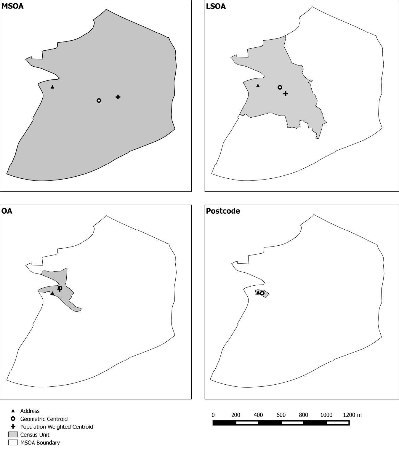
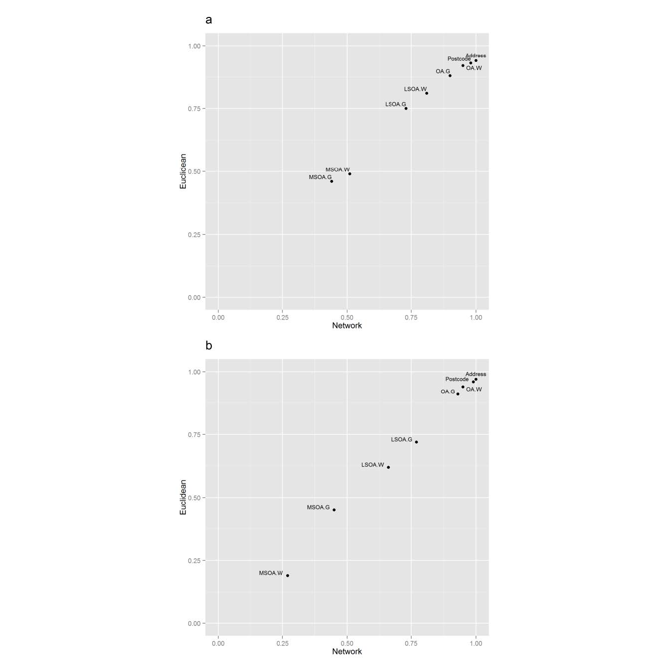
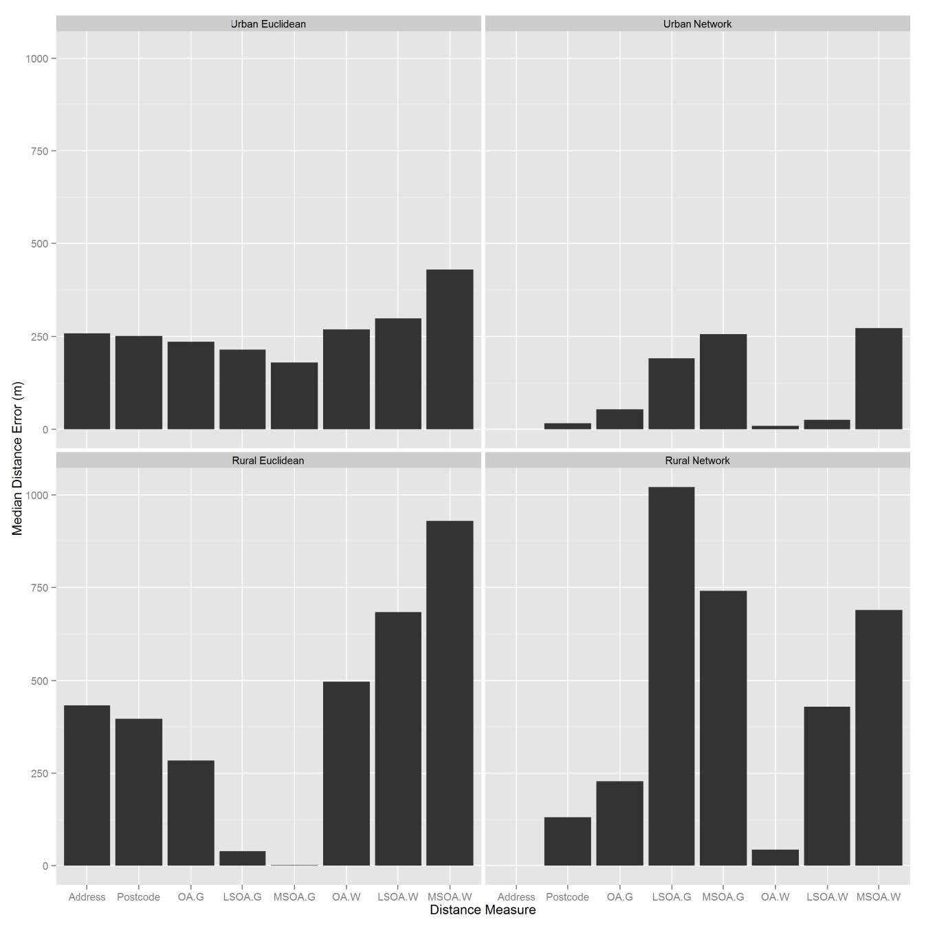
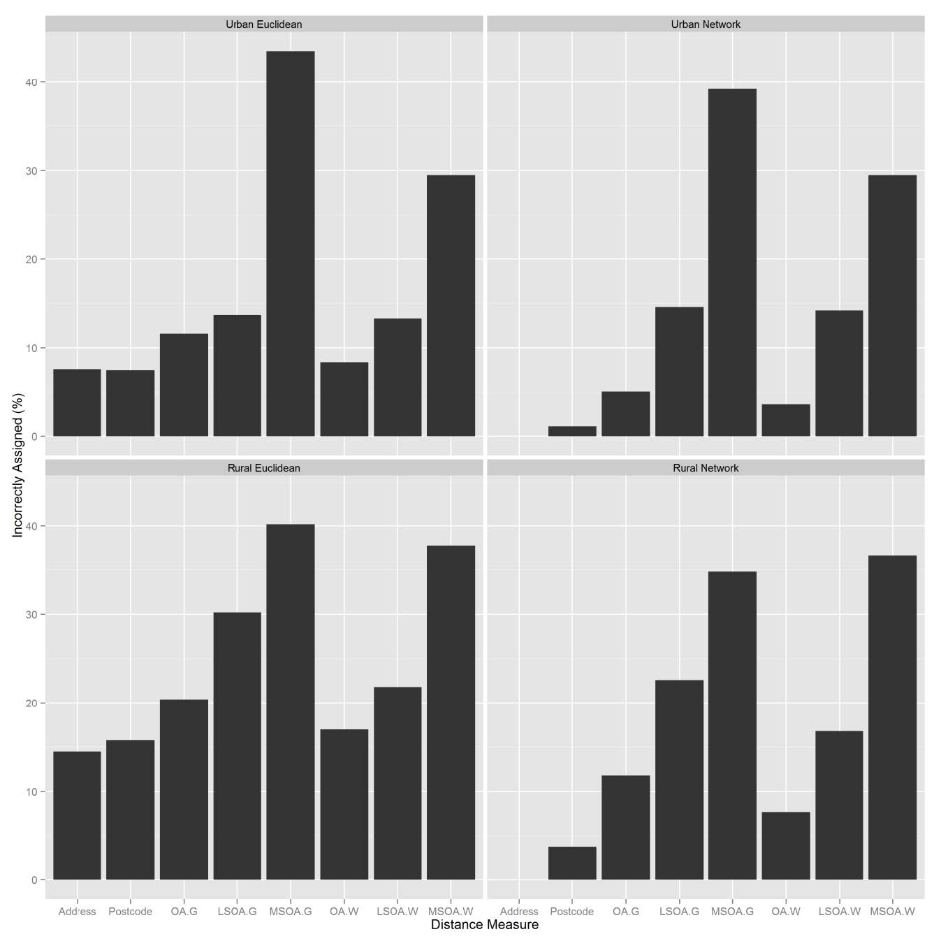
1. | Raghunath Kodi, Mohana Ramana Ravuri, V. Veeranna, M. Ijaz Khan, Sherzod Abdullaev, Nissren Tamam, Hall current and thermal radiation effects of 3D rotating hybrid nanofluid reactive flow via stretched plate with internal heat absorption, 2023, 53, 22113797, 106915, 10.1016/j.rinp.2023.106915 | |
2. | Mohd Ahtesham Hussain Siddiqui, Somnath Chattopadhyaya, Shubham Sharma, Changhe Li, Yanbin Zhang, Anita Gehlot, Abhinav Kumar, Fuad A. Awwad, M. Ijaz Khan, Emad A. A. Ismail, Underground Coal Mines Unexplored Strata Structure Identification with Subsurface Profiling: A Case Study of Inherent Fault-Detection Method, 2024, 41, 2524-3462, 2357, 10.1007/s42461-024-00992-6 | |
3. | M. Venkata Subba Rao, Kotha Gangadhar, Ali J. Chamkha, MHD Eyring-Powell fluid flow over a stratified stretching sheet immersed in a porous medium through mixed convection and viscous dissipation, 2023, 0228-6203, 1, 10.1080/02286203.2023.2296678 | |
4. | Muhammad Naveed Khan, Mostafa A. Hussien, F.M. Allehiany, N. Ameer Ahammad, Zhentao Wang, Ebrahem A. Algehyne, Variable fluid properties and concentration species analysis of a chemically reactive flow of micropolar fluid between two plates in a rotating frame with cross diffusion theory, 2023, 189, 0301679X, 108943, 10.1016/j.triboint.2023.108943 | |
5. | Mohd Ahtesham Hussain Siddiqui, Somnath Chattopadhyaya, Shubham Sharma, Changhe Li, Yanbin Zhang, Abhinav Kumar, Dražan Kozak, Mohamed Abbas, Jasmina Lozanovic, Productivity enhancement of continuous miners packages of underground mines with energy conservation in industrial sectors, 2024, 0144-5987, 10.1177/01445987241266084 | |
6. | Mohd Ahtesham Hussain Siddiqui, Shahzad Akhtar, Somnath Chattopadhyaya, Shubham Sharma, Abhinav Kumar, Mohamed Abbas, 611 Universal Drilling Machine Reliability Modeling and Performance Evaluation in Subterranean Coal Mines, 2024, 57, 0723-2632, 3559, 10.1007/s00603-023-03705-5 | |
7. | Jing Zhang, Rubing Chen, Lingfa Lu, Jinjiang Yuan, Two-agent scheduling of equal-length jobs on uniform parallel machines, 2025, 0, 1547-5816, 0, 10.3934/jimo.2025031 |