Research article

Dynamical behaviour of fractional-order atmosphere-soil-land plant carbon cycle system

  • Received: 03 October 2019 Accepted: 13 January 2020 Published: 21 January 2020
  • MSC : 34A08, 37N25

  • The terrestrial carbon cycle is the most important constitution and plays a prominent role in the global carbon cycle. This paper investigates the dynamical behaviours and mathematical properties of a time fractional-order atmosphere-soil-land plant carbon cycle system. We give a sufficient condition for existence and uniqueness of the solution, and obtain the conditions for local asymptotically stable of the equilibrium points by using fractional Routh-Hurwitz stability conditions. Furthermore, we introduce a discretization process to discretize this fractional-order system, and study the necessary and sufficient conditions of stability of the discretization system. It shows that the stability of the discretization system is impacted by the system's fractional parameter. Numerical simulations show the richer dynamical behaviours of the fractional-order system and verify the theoretical results.

    Citation: Wenjun Liu, Zhijing Chen. Dynamical behaviour of fractional-order atmosphere-soil-land plant carbon cycle system[J]. AIMS Mathematics, 2020, 5(2): 1532-1549. doi: 10.3934/math.2020105

    Related Papers:

    [1] Muhammad Bilal Riaz, Nauman Raza, Jan Martinovic, Abu Bakar, Osman Tunç . Modeling and simulations for the mitigation of atmospheric carbon dioxide through forest management programs. AIMS Mathematics, 2024, 9(8): 22712-22742. doi: 10.3934/math.20241107
    [2] M. Mossa Al-Sawalha, Humaira Yasmin, Ali M. Mahnashi . Kink phenomena of the time-space fractional Oskolkov equation. AIMS Mathematics, 2024, 9(11): 31163-31179. doi: 10.3934/math.20241502
    [3] Hasib Khan, Jehad Alzabut, Anwar Shah, Sina Etemad, Shahram Rezapour, Choonkil Park . A study on the fractal-fractional tobacco smoking model. AIMS Mathematics, 2022, 7(8): 13887-13909. doi: 10.3934/math.2022767
    [4] Abdulaziz Khalid Alsharidi, Saima Rashid, S. K. Elagan . Short-memory discrete fractional difference equation wind turbine model and its inferential control of a chaotic permanent magnet synchronous transformer in time-scale analysis. AIMS Mathematics, 2023, 8(8): 19097-19120. doi: 10.3934/math.2023975
    [5] Rashid Jan, Sultan Alyobi, Mustafa Inc, Ali Saleh Alshomrani, Muhammad Farooq . A robust study of the transmission dynamics of malaria through non-local and non-singular kernel. AIMS Mathematics, 2023, 8(4): 7618-7640. doi: 10.3934/math.2023382
    [6] Abeer Al Elaiw, Murugesan Manigandan, Muath Awadalla, Kinda Abuasbeh . Existence results by Mönch's fixed point theorem for a tripled system of sequential fractional differential equations. AIMS Mathematics, 2023, 8(2): 3969-3996. doi: 10.3934/math.2023199
    [7] P. Veeresha, D. G. Prakasha, Jagdev Singh . Solution for fractional forced KdV equation using fractional natural decomposition method. AIMS Mathematics, 2020, 5(2): 798-810. doi: 10.3934/math.2020054
    [8] Devendra Kumar, Jogendra Singh, Dumitru Baleanu . Dynamical and computational analysis of a fractional predator-prey model with an infectious disease and harvesting policy. AIMS Mathematics, 2024, 9(12): 36082-36101. doi: 10.3934/math.20241712
    [9] Maysaa Al-Qureshi, Saima Rashid, Fahd Jarad, Mohammed Shaaf Alharthi . Dynamical behavior of a stochastic highly pathogenic avian influenza A (HPAI) epidemic model via piecewise fractional differential technique. AIMS Mathematics, 2023, 8(1): 1737-1756. doi: 10.3934/math.2023089
    [10] Mohamed Lamine Sahari, Abdel-Kaddous Taha, Louis Randriamihamison . Exploring three periodic point dynamics in 2D spatiotemporal discrete systems. AIMS Mathematics, 2025, 10(3): 5021-5051. doi: 10.3934/math.2025230
  • The terrestrial carbon cycle is the most important constitution and plays a prominent role in the global carbon cycle. This paper investigates the dynamical behaviours and mathematical properties of a time fractional-order atmosphere-soil-land plant carbon cycle system. We give a sufficient condition for existence and uniqueness of the solution, and obtain the conditions for local asymptotically stable of the equilibrium points by using fractional Routh-Hurwitz stability conditions. Furthermore, we introduce a discretization process to discretize this fractional-order system, and study the necessary and sufficient conditions of stability of the discretization system. It shows that the stability of the discretization system is impacted by the system's fractional parameter. Numerical simulations show the richer dynamical behaviours of the fractional-order system and verify the theoretical results.


    From the researches and reports in recent years, it has been known that the earth is confronting with environmental pollution and energy crisis and people from all walks of life are trying hard to find solutions. The most important point is to understand the process of terrestrial carbon cycle, which plays the prominent position in the global carbon cycle. In different fields, theoretical issues concerning the carbon cycle have been studied differently, such as in atmosphere science [1], ocean science [2,3], forest ecological system [4], geological sciences [5] and so on [6,7]. Research achievements mainly concentrate on the carbon source and sink, carbon footprint and carbon exchange. This study established a dynamical system to investigate the evolution of the carbon cycle.

    Carbon cycle change, increases in the NOx emission to the atmosphere and in the atmospheric aerosol (Black carbon, PM2.5 etc) amount, will perturb the Earth's radiative budget and exert large impact on the Earth’s climate. In [8], Leonid et al. proposed a terrestrial ecosystem carbon life cycle model to investigate the intensity of carbon source and sink. Enting[9] used Laplace transform to analyze the carbon cycle. Michela et al. [10] built a carbon cycle dynamic system for Italy, Siena province and examined the carbon footprint of six carbon emission scenarios. Pan et al. [11] estimated the global forest carbon balance and Piao et al. [12] described China's carbon budget and its change mechanism by remote sensing data and a biogeochemical model. According on China's regional terrestrial ecosystem carbon cycle, Fu et al. [13] studied regional atmosphere-soil-land plant carbon cycle system based on the analysis of the carbon flux. The dynamic behaviour of the system is studied from the point of view of stability.

    On the other hand, fractional-order calculus has gained much popularity from theoretical as well as application viewpoints. It used to be considered as the generalization of classical integer-order calculus to real or complex order. Compared with integer calculus, the major merit of fractional calculus lies in the fact that it has memory. Many people are interested in developing the theoretical analysis and numerical methods for fractional-order differential equations. Actually, fractional-order differential equations have recently proved to be an effective and valuable measures in various fields such as in engineering [14,15,16,17], physics [18,38], mathematical biology [19,20,21], psychological and life sciences [22,23,24,25,26] and other scientific fields. Furthermore, more and more researchers have performed investigation to study the mathematical properties and numerical solutions of the fractional-order ecological system recently. In [19], Ahmed et al. investigated the fractional-order predator-prey system and the fractional-order rabies system to obtain the existence and uniqueness of solutions, the stability of equilibrium points and numerical solutions for these systems. In [26], authors showed us fractional-order energy demand-supply system which confirmed the energy resource attractor with a necessary condition about the existence of chaotic behaviors and two different control strategies. In song et al. [27], a fractional-order delayed predator-prey system was proposed and analyzed. The main work is investigating the stability of the system. Furthermore, the authors find that fractional-order can affect the stability of the system without harvesting terms.

    We here want to make a more precise depiction to the atmosphere-soil-land plant carbon cycle by using the time fractional differential operator which lies in the system itself that the memory data of it. It can characterize the real cycle which also affected by the history. Therefore, by investigating this system, we may have a better perception and the performer could refer to our result to make some change when facing some environmental problem. Based on the above analysis, we consider a class of fractional-order differential system to describe the dynamics of atmosphere-soil-land plant carbon cycle. The system consists of x1(t), x2(t) and x3(t), where x1(t) is the time-dependent variable of carbon flux in atmosphere, x2(t) is the carbon flux of soil and x3(t) is the carbon flux of animals and plants. According to the law of carbon flow, we give the following assumptions:

    Assumption 1: in order to maintain a balance, the inflow and outflow is equal to the total carbon flow.

    Assumption 2: the internal carbon flux is determined by the carbon flow of three cycles (atmosphere cycle, soil cycle and land plant cycle).

    Assumption 3: the internal flow of each cycle obeys the rules of supply pattern, receive pattern, Lotka-Volterra pattern and diffusion pattern.

    Assumption 4: the rest of carbon flow is ignored except the large carbon flow changed in the atmosphere-soil-land cycle.

    On the basis of Assumptions 1–4, we could build the atmosphere-soil-land plant terrestrial ecosystem carbon cycle dynamic system as shown in Figure 1.

    Figure 1.  Atmosphere-soil-land plant carbon cycle system.

    In this paper, we assume the carbon inflow q1 of the atmosphere cycle and the carbon inflow q2 of the soil cycle are both constant.

    From Figure 1, it shows that a part of carbon flow escapes out with the change of natural phenomenon in the atmosphere cycle and this carbon flow represents the release of carbon dioxide from the atmosphere under the combined action of the atmosphere cycle and the land plant cycle ultimately. And some of it flows into soil cycle by carbon dioxide fixation. What's more, in the soil cycle, a part of carbon flow sinks into the atmosphere cycle by breath and decomposition and another part of it goes out with deposition. In the land plant cycle, a part of carbon flow flows into the atmosphere cycle by breath and burning and another part of it goes into the soil cycle by decomposition.

    Under the premise of the above hypothesis and Figure 1, the three-dimensional fractional-order atmosphere-soil-land plant carbon cycle system is obtained as follows:

    dαx1dtα=q1m1x1β12x2+α21x2β1x3(1x3A1),dαx2dtα=q2m2x2+β12x2α21x2+α32x3α22A2β2x1,dαx3dtα=(α32+α31)x3+γ31x1x3, (1.1)

    where α is the fractional order satisfying 0<α1 and dαdtα is in the sense of the Caputo fractional derivative, and the coefficients of the system have specific meanings: mi (i=1,2) are the carbon outflow coefficients; Ai (i=1,2) are the positive constants; β12 is the receive coefficient of carbon flow from the atmosphere cycle to the soil cycle; α21 is the supply coefficient of carbon flow from the soil cycle to the atmosphere; β1 is the diffusion coefficient of the atmosphere cycle that depends on the carbon reserve of the land plant cycle; α32 is the supply coefficient of carbon flow from the land plant cycle to the soil cycle; α22 is the diffusion coefficient of the soil cycle; β2 is the diffusion coefficient of the soil cycle that depends on the carbon reserve of the atmosphere cycle; α32 is the supply coefficient of carbon flow from the land plant cycle to the soil cycle; α31 is the supply coefficient of carbon flow from the land plant cycle to the atmosphere cycle; γ31 is the Lotka-Volterra coefficient of carbon flow from the land plant cycle to the atmosphere cycle.

    A simplified formula is

    dαx1dtα=q1m1x1+α1x2β1x3(1x3K1),dαx2dtα=q2β2x1+α2x2+α3(x3K2),dαx3dtα=α4x3+γ1x1x3, (1.2)

    where α1=α21β12, K1=A1, α2=β12m2α21, α3=α32, K2=α22α32A2, α4=α32+α31, γ1=γ31. System (1.2) reflects the interactive relationships among the atmosphere cycle, soil cycle and land plant cycle. In the above system, there are complicated dynamics existing between the variables and parameters. In addition, it is beneficial to us for more intuitive analysis of the system.

    In this article, we first put forward a fractional-order system of atmosphere-soil-land plant carbon cycle. Moreover, to show more realistic conditions, we give system parameter estimation method. Then we discuss the sufficient condition for existence and uniqueness of the solution. And the conditions of local stability of the fractional-order system are analyze by calculating equilibrium points. We also find the existence of the asymptotically stable attractor of the system and the carbon cycle in the planet is balanced by numerical simulations. Furthermore, we construct a discretization process of fractional-order system and study the necessary and sufficient conditions of the stability of the discretization system. It shows that the fractional-order parameter has an impact on the stability of the discretization system.

    This paper is arranged as follows. Section 2 analyzes the sufficient condition for existence and uniqueness of the solution of the fractional-order atmosphere-soil-land plant carbon cycle system and investigates conditions of the local stability of the system. Section 3 discretizes the fractional-order atmosphere-soil-land plant carbon cycle system and analyzes the necessary and sufficient conditions of stability of discretization system. We use numerical simulations which not only illustrate our results with the theoretical analysis, but also exhibit the complex dynamical behaviors in Section 2 and Section 3, respectively.

    In this section, we use a class of fractional-order differential system called atmosphere-soil-land plant carbon cycle system to analyze the carbon flux relationship among the atmosphere cycle, the soil cycle and the land plant cycle.

    The Caputo definition of fractional derivative [28] is given as

    Dαf(t)=Jlαf(l)(t),α>0,

    where the operator Dα is referred as the ``α-order Caputo differential operator", f(l) represents the l-order derivative of f(t), l is the smallest integer which is not less than α and Jθ is the θ-order Riemann-Liouville integral operator which can be described as

    Jθu(t)=1Γ(θ)t0(tτ)(θ1)u(τ)d(τ),θ>0,

    where Γ(θ) is the Euler's Gamma function.

    In [29,30,31,32,33], stability conditions and their applications to systems of fraction-order differential equations were reported. We consider the following nonlinear autonomous fractional-order system

    DαX(t)=F(X(t)),X(0)=X0, (2.1)

    where X(t)=(x1,x2,x3)TR3, F:R3R3 is a nonlinear vector function in terms of X. The Jacobian matrix evaluated at the equilibrium point X=(x1,x2,x3) is

    J(X)=(Fixj)ij|x=x.

    The local stability of the equilibrium points of a linearized fractional-order system can be obtained from the following lemma [29] :

    Lemma 2.1. If all the eigenvalues λ1,λ2,λ3 of the equilibrium point X of system (2.1), satisfy the Matignon's conditions [30] which can be described as

    |argλi|>απ/2,(i=1,2,3), (2.2)

    where |argλi|(i=1,2,3) denotes the argument value of the eigenvalue λi. Then X is locally asymptotically stable.

    The fractional-order atmosphere-soil-land plant carbon cycle system can be written in the following form

    DαX(t)=F(X(t)),t(0,T),X(0)=X0,

    where

    F(X)=(q1m1x1+α1x2β1x3(1x3K1)q2β2x1+α2x2+α3(x3K2)α4x3+γ1x1x3).X=(x1,x2,x3)T,X0=(x10,x20,x30)T

    Define the supermum norm as

    N=sup|N(t)|,t(0,T]

    then, the norm of the matrix M=[mij[t]] is defined by [35]

    M=i,jsup|mij[t]|,t(0,T].

    We investigate the existence and uniqueness of the solution in the region Ω×(0,T] where

    Ω={(x1,x2,x3:max(|x1|,|x2|,|x3|)ξ},

    thus, we get the solution of the system as follows

    X=X0+1Γ(α)t0(tτ)α1F(X(τ))dτ=H(X),

    so

    H(X1)H(X2)=1Γ(α)t0(tτ)α1F(X1(τ)X2(τ))dτ.

    Finally, according to the above conditions, we get the following inequality

    H(X1)H(X2)TαΓ(α+1)max{m1,α2,α4γ1ξexpγ1ξ}X1X2LX1X2,

    where

    L=TαΓ(α+1)max{m1,α2,α4γ1ξexpγ1ξ}.

    If L<1, then the mapping X=H(X) is a contraction mapping and we get the sufficient condition for existence and uniqueness of the solution of system as follows.

    Theorem 2.1. The sufficient condition for existence and uniqueness of the solution of system in the region Ω×(0,T] with initial conditions X(0)=X0 and t(0,T) is

    L=TαΓ(α+1)max{m1,α2,α4γ1ξexpγ1ξ}<1.

    In the practical application, it is very important to estimate parameters of the system. Next, we give a simple estimation method for the various parameters involved in the system.

    (i) Estimate of the coefficients of diffusion β1, β2.

    We use the following formulas to estimate the diffusion coefficients.

    β1=ν1ω1,β2=η1ξ1,

    where ν1 represents the quantity of diffusion in the atmosphere cycle, ω1 represents the total carbon dioxide, η1 represents the total quality of diffusion in the soil cycle, ξ1 represents the total carbon dioxide.

    (ii) Estimate of the coefficient of supply α1,2,3,4 and the Lotka-Volterra coefficient γ1.

    In the case of α1. Let x1(0)=0, when t is small, we ignore the role of carbon in atmosphere cycle and land plant cycle, and the approximate assumption x2=x21, then the first formula in system (1.2) becomes

    ˙x1=α1x21.

    So, when t=t1, x1=x21, then from the above formula, we get

    α11=t1,

    thus, the above formula implies that: in the case of a certain speed of carbon in atmosphere cycle, α11 equals the time which carbon supply becomes 0 required. So, estimation of the supply coefficient, we can convert to estimate from the time perspective.

    (iii) Estimation of the parameter q1, m1, K1, q2, K2.

    According to statistical data fitting, we can get the estimated value of q1, m1, K1, q2, K2.

    To analyze system and discuss the stability of the system, we first find out the equilibrium points of system (1.2). Let

    dαx1dtα=0,dαx2dtα=0,dαx3dtα=0.

    After calculating, the system has three equilibrium points

    E0=(α1α3K2α1q2+α2q1α1β2+α2m1q1α1+m1α1(α1α3K2β2q2+α2q1α1β2+α2m1)0)T,E1=(¯x11,¯x21,¯x31),E2=(¯x12,¯x22,¯x32). (2.3)

    For system (1.2), the Jacobian matrix of equilibrium point (x,y,z) is as below

    J(x,y,z)=(m1α1β1+2β1K1zβ2α2α3γ1z0α4+γ1x).

    Theorem 2.2. The atmosphere cycle and soil cycle equilibrium point E0=(α1α3K2α1q2+α2q1α1β2+α2m1,q1α1+m1α1(α1α3K2β2q2+α2q1α1β2+α2m1),0) is locally asymptotically stable if α4>γ1α1α3K2α1q2+α2q1α1β2+α2m1, α2<m1 and m1α2α1β2<0.

    Proof. The Jacobian matrix of equilibrium point E0 is

    J(E0)=(m1α1β1β2α2α300α4+γ1α1α3K2α1q2+α2q1α1β2+α2m1).

    The corresponding characteristic polynomial is

    f(λ)=[λ(α4+γ1α1α3K2α1q2+α2q1α1β2+α2m1)]×[(λ+m1)(λα2)+α1β2].

    So the eigenvalues of the Jacobian matrix J(E0) are

    λ1,2=α2m12±12(m1+α2)24α1β2,λ3=α4+γ1α1α3K2α1q2+α2q1α1β2+α2m1.

    If α2<m1 and m1α2α1β2<0, then both eigenvalues λ1,2 are negative. If α4>γ1α1α3K2α1q2+α2q1α1β2+α2m1, then λ3 is negative. Therefore, all the eigenvalues of the atmosphere cycle and soil cycle equilibrium point E0 satisfy Matignon's conditions (2.2).

    Next, the eigenvalues of the two-species equilibrium points E1 and E2 are given by

    P(λ)=λ3+A1λ2+A2λ+A3=0,

    where

    A1=m1α2+α4β1¯x1;A2=(α4γ1¯x2)(m1α2)m1α2+α1β2+γ1¯x3(β12β1¯x3K1);A3=(α4β2¯x2)(m1α2α1β2)γ1¯x3(α1α3+m1(β12β1¯x3K1))+γ1¯x3(m1α2)(β12β1¯x3K1).

    Remark 2.1. Since E0 is a land plant free equilibrium and the discriminant of eigenvalues is greater than zero, which verifies the first statement in Theorem 2.3, we notice that the conditions of Theorem 2.2 is free with the order α.

    Now, we use the following theorem to determine the local stability of interior equilibrium points E1 and E2.

    Theorem 2.3. [29] If the discriminant of the eigenvalues of equation (2.3.1) is given as

    D(P)=18A1A2A3+(A1A2)24A3(A1)34(A2)327(A3)2,

    then equilibrium points E1 and E2 are locally asymptotically stable if they satisfy the following fractional Routh-Hurwitz conditions:

    (i) If D(P)>0, then the necessary and sufficient condition for equilibrium point E1(E2), to be locally asymptotically stable, is A1>0, A3>0, A1A2A3>0.

    (ii) If D(P)<0, A10, A20, A3>0, then E1(E2) is locally asymptotically stable for α<23. However, if D(P)<0, A1<0, A2<0, α>23, then all roots of equation (2.3.1) satisfy the condition |arg(λ)|<απ/2.

    (iii) If D(P)<0, A1>0, A2>0, A1A2A3=0, then E1(E2) is locally asymptotically stable for all α(0,1).

    (iv) The necessary condition for equilibrium point E1(E2), to be locally asymptotically stable, is A3>0.

    In this subsection, to briefly illustrate the system dynamics, we use a modified Adams-Bashforth-Moulton algorithm method proposed by [34] to solve the system. The numerical simulation results show that there is a rather complex nonlinear relationship among the atmosphere cycle, soil cycle and land plant cycle. As in [13], we select the following parameter values: q1=0.1, m1=0.03, α1=0.06, β1=0.02, K1=0.13, q2=0.15, β2=0.02, α2=0.02, α3=0.02, K2=0.25, α4=0.02, γ1=0.0005. Then numerical simulations are performed for α=0.88, 0.94, 0.97, and 0.99. As can be seen from Figure 2, the dynamic behavior of the system has obvious differences under different values. When α=0.88 and 0.94, an asymptotically stable attractor exists in Figure 2(a) and (b). When fractional-order parameter α is bigger, the speed of asymptotically stable of the system is faster. When α=0.97 and 0.99, Figure 2 (c) and (d) show that the system has a stable limit cycle. Therefore, different fractional-order parameters α have different effects on the atmosphere-soil-land plant system. In addition, by observing the relationship among variables with time, we get Figure 3. From Figure 3, we find that the carbon reserve of the atmosphere has a maximum value with time and then keeps steady; the carbon reserve of the soil also has a maximum value with time, then it has a steady level; and the carbon reserve of the land plant cycle decreases to a minimal level and keeps steady finally. It shows that the carbon flow keeps a balance in the atmosphere cycle, soil cycle and land plant cycle.

    Figure 2.  Phase diagrams for system using the fixed parameter values and fractional orders: α=0.88 (asymptotically stable), α=0.94 (asymptotically stable), α=0.97 (limit cycle), α=0.99 (limit cycle).
    Figure 3.  The evolution over time of atmosphere-soil-land plant carbon cycle.

    In the following, we adopt the discretization [26,35] of fractional-order atmosphere-soil-land plant carbon cycle dynamic system and investigate the necessary and sufficient conditions for the stabilization of discretized system.

    Now, we assume that x1(0)=x10,x2(0)=x20,x3(0)=x30 are the initial values of system (1.2). So the discretization process of fractional-order atmosphere-soil-land plant carbon cycle dynamic system (1.2) with piecewise constant arguments is given as [35]

    Dαx1(t)=q1m1x1([ts]s)+α1x2([ts]s)β1x3([ts]s)(1x3([ts]s)K1),Dαx2(t)=q2β2x1([ts]s)+α2x2([ts]s)+α3(x3([ts]s)K2),Dαx3(t)=α4x3([ts]s)+γ1x1([ts]s)x3([ts]s). (3.1)

    Firstly, let t[0,s), so ts[0,1), we obtain

    Dαx1(t)=q1m1x10+α1x20β1x30(1x30K1),Dαx2(t)=q2β2x10+α2x20+α3(x30K2),Dαx3(t)=α4x30+γ1x10x30, (3.2)

    and the solution of (3.2) is reduced to

    x11(t)=x10+Iα[q1m1x10+α1x20β1x30(1x30K1)]=x10+tααΓ(α)[q1m1x10+α1x20β1x30(1x30K1)],x21(t)=x20+Iα[q2β2x10+α2x20+α3(x30K2)]=x20+tααΓ(α)[q2β2x10+α2x20+α3(x30K2)],x31(t)=x30+Iα(α4x30+γ1x10x30)=x30+tααΓ(α)(α4x30+γ1x10x30). (3.3)

    where Iα=tααΓ(α).

    Secondly, let t[s,2s), so ts[1,2), we get

    Dαx1(t)=q1m1x11+α2x21β1x31(1x31K1),Dαx2(t)=q2β2x11+α2x21+α3(x31K2),Dαx3(t)=α4x31+γ1x11x31,

    which has the following solution

    x12(t)=x11(s)+Iα[q1m1x11(s)+α1x21(s)β1x31(s)(1x31(s)K1)]=x11(s)+(ts)ααΓ(α)[q1m1x11(s)+α1x21(s)β1x31(s)(1x31(s)K1)],x22(t)=x21(s)+Iα[q2β2x11(s)+α2x21(s)+α3(x31(s)K2)]=x21(s)+(ts)ααΓ(α)[q2β2x11(s)+α2x21(s)+α3(x31(s)K2)],x32(t)=x31(s)+Iα[α4x31(s)+γ1x11(s)x31(s)]=x31(s)+(ts)ααΓ(α)[α4x31(s)+γ1x11(s)x31(s)].

    So, after repeating the discretization process n times, we gain

    x1n+1(t)=x1n(ns)+(tns)ααΓ(α)[q1m1x11(ns)+α1x21(ns)β1x31(ns)(1x31(ns)K1)],x2n+1(t)=x2n(ns)+(tns)ααΓ(α)[q2β2x11(ns)+α2x21(ns)+α3(x31(ns)K2)],x3n+1(t)=x3n(ns)+(tns)ααΓ(α)[α4x31(ns)+γ1x11(ns)x31(ns)], (3.4)

    where t[ns,(n+1)s). For t(n+1)s, system (3.4) is simplified to

    x1n+1=x1n+sααΓ(α)[q1m1x1n+α1x2nβ1x3n(1x3nK1)],x2n+1=x2n+sααΓ(α)[q2β2x1n+α2x2n+α3(x3nK2)],x3n+1=x3n+sααΓ(α)(α4x3n+γ1x1nx3n). (3.5)

    In what follows, we discuss the asymptotic stability of system (1.2) at the fixed equilibrium points. By considering the Jacobian matrix of these fixed points and calculating their eigenvalues, the local stability of these points based on the roots of the system's characteristic equation [36] is studied. The Jacobian matrix of system (3.5) is given by

    J(x1n,x2n,x3n)=(1+sααΓ(α)(m1)sααΓ(α)α1sααΓ(α)(β1+2β1x3nK1)sααΓ(α)(β2)1+sααΓ(α)α2SααΓ(α)α3sααΓ(α)γ1x3n01+sααΓ(α)(α4+γ1x1n)). (3.6)

    Theorem 3.1. The fixed points E0 of system (3.5) is locally asymptotically stable if and only if

    0<α4+γ1α1α3K2α1q2+α2q1α1β2+α2m1<2αΓ(α)sα,

    and one of the following conditions holds:

    (i) ϕ22=ψ and 4<sααΓ(α)ϕ1<0;

    (ii) ϕ22>ψ and 4<sααΓ(α)(ϕ1±ϕ22ψ)<0;

    (iii) ϕ22<ψ and ϕ1+sα4αΓ(α)(ϕ21+ψϕ22)<0,

    where

    ϕ1=α2m1,β2=m1+α2,ψ=4α1β2.

    Proof. The Jacobian matrix evaluated at E0 is given by

    J(E0)=(1+sααΓ(α)(m1)sααΓ(α)α1sααΓ(α)(β1)sααΓ(α)(β2)1+sααΓ(α)α2SααΓ(α)α3001+sααΓ(α)(α4+γ1ϑ)).

    where ϑ=α1α3K2α1q2+α2q1α1β2+α2m1.

    The eigenvalues of J(E1) are

    λ1=1+sααΓ(α)(α4+γ1α1α3K2α1q2+α2q1α1β2+α2m1),λ2,3=1+sα2αΓ(α)(α2m1±(m1+α2)24α1β2).

    So if the fixed point E0 is locally asymptotically stable, it satisfies the stability conditions |λ1|<1 and |λ2,3|<1 by the postulates in this theorem.

    Next, let us discuss the stability of fixed points E1,2. To simplify calculations, we get the Jacobian matrix of these fixed points

    J(E1,2)=(γ11γ12γ13γ21γ22γ23γ31γ32γ33),

    where

    γ11=1+sααΓ(α)(m1),γ12=sααΓ(α)α1,γ13=sααΓ(α)(β1+2β1K1¯x3i),γ21=sααΓ(α)β2γ22=1+sααΓ(α)α2,γ23=sααΓ(α)α3,γ31=sααΓ(α)γ1¯x3i,γ32=0,γ33=1+sααΓ(α)(α4+γ1¯x3i) (3.7)

    and variables ¯x1i, ¯x2i, ¯x3i, i=0,1,2 are defined by equation (2.3). The characteristic equation of J(E1,2) is expressed as follows:

    f(λ)=λ3+K1λ2+K2λ+K3=0,

    with the coefficients

    K1=V1V5V73,K2=V1(V5+V7)U2V3V2V42K13,K3=U2(V2V6+V3V5)+V7(V2V4V1V5V5)K2K11, (3.8)

    where

    U1=sααΓ(α)2β1¯x3iK1, U2=sααΓ(α)γ1¯x3i, U3=sααΓ(α)γ1¯x1i,

    V1=sααΓ(α)(m1), V2=sααΓ(α)α1,

    V3=sααΓ(α)(β1)U1, V4=sααΓ(α)(β2),

    V5=sααΓ(α)α2, V6=sααΓ(α)α3,

    V7=sααΓ(α)(α4)+U3.

    According to the Jury's criterion [37], if fixed points E1,2 are locally asymptotically stable, they should satisfy the following conditions:

    1+K1+K2+K3>0, 1K1+K2K3>0,

    1K2+K1K3K23>0, 1+K2K1K3K23>0.

    Therefore, the above conditions indicate that fixed points E1,2 are locally asymptotically stable if the system's parameters belong to the following set

    {H:[CBA1]Ωi,i=1,2,3}

    where

    H=(α1,α2,α3,α4,α5,β1,β2,α,s),

    Ω1=(A3+(A24B)2A+12,A3(A24B)2A+12),

    Ω2=(BA1,B+3A+7),

    Ω3=(A+3+A2+4B+14A+232,A+3A2+4B+14A+232),

    A=V1(V5+V7),

    B=V1(V5+V7)U2V3V2V4,

    C=U2(V2V6+V3V5)V7(V2V4V1V5V5).

    Discretization is a new method to analyze the fractional-order system. For discretized system, we mainly consider the stability of the fixed points of the system. However, even if we can obtain analytical conditions about stability, it would be a little difficult to deal with them thoroughly by theory.

    So, in order to analyze the stability of the fixed points, we adopt numerical simulations to study the global dynamical behaviours of system (3.5). In the simulation process, some dynamical behaviours of system (3.5) can be shown, for example asymptotic behaviours near the equilibrium points and the stable limit cycle. In the following, we will find that when fractional-order parameters α and s with different values, it will have strong effect on the stability of system (3.5).

    First, as in [13], we fix parameters q1, m1, α1, β1, K1, q2, β2, α2, α3, K2, α4, γ1. Then we vary parameters α and s. On the basis of the above-mentioned parameters values and setting α=0.9, α=0.98 and s=0.6, we get Figure 4(a) and (b) which depicts the phase portraits of the system (3.5). When α=0.9, α=0.98 and s=0.4, we gain Figure 4(c) and (d). In the case of Figure 4(a)-(d), discretized system (3.5) is similar with fractional-order system (1.2) under increasing fractional-order parameter α and fixing parameter s. When α=0.9,0.98 and s=0.09, the phase portraits of system (3.5) are depicted in Figure 4(e)-(f), respectively. From Figure 4(c)-(f), we notice that increasing parameter s and decreasing fractional-order parameter α make the behavior of system (3.5) stable. And when α=0.3,0.5 and s=0.09, Figure 4(g)-(h) shows that the stable limit cycle of system (3.5) which confirms the above result; because it is shown that the above result is reversible when s is small and decreasing fractional-order parameter α destabilize the stable behaviour of system (3.5).

    Figure 4.  Trajectory of the system (3.5) in phase space when the coefficient are fixed and (a) α = 0.9, s=0.6; (b) α=0.98, s=0.6; (c) α=0.9, s=0.4; (d) α=0.98, s=0.4; (e) α=0.9, s=0.09; (f) α=0.98, s=0.09; (g) α=0.3, s=0.09; (h) α=0.5, s=0.09.

    In this paper, we introduced the fractional-order atmosphere-soil-land plant carbon cycle system and adopted discretization method to discretize this system. We analyzed some dynamic behaviours of the fractional-order atmosphere-soil-land plant carbon cycle system. We obtained the sufficient condition for existence and uniqueness of the solution and the conditions of local stability of the equilibrium points of the fractional-order system. Furthermore, for discretization system, the necessary and sufficient conditions of stability of the discretization system were also obtained. In discretization system, we knew that when applying the discretization process on fractional-order atmosphere-soil-land plant carbon cycle system as α1, the discretization would be Euler's process. In addition, we found that, the stability of the discretization system were impacted by the fractional parameter. Numerical Simulations verified the correctness of our results.

    This work was supported by the National Natural Science Foundation of China (Grant No. 11771216), the Major Program of the National Social Science Fund of China (Grant No. 17ZDA092), the Key Research and Development Program of Jiangsu Province (Social Development) [grant number BE2019725], the Six Talent Peaks Project in Jiangsu Province (Grant No. 2015-XCL-020), the Qing Lan Project of Jiangsu Province and the Laboratory Open Project of NUIST.

    The authors state that there is no conflict of interest.


    [1] M. Reichstein, M. Bahn, P. Ciais, et al. Climate extremes and the carbon cycle, Nature, 500 (2013), 287-295. doi: 10.1038/nature12350
    [2] S. Honjo, T. I. Eglinton, C. D. Taylor, et al. Understanding the Role of the Biological Pump in the Global Carbon Cycle: An Imperative for Ocean Science, Oceanography, 27 (2014), 10-16.
    [3] L. G. Anderson, R. W. Macdonald, Observing the Arctic Ocean carbon cycle in a changing environment, Polar Res., 34 (2015), 26891.
    [4] A. Ito, Modelling of carbon cycle and fire regime in an east Siberian larch forest, Ecol. Model., 187 (2005), 121-139. doi: 10.1016/j.ecolmodel.2005.01.037
    [5] R. Causebrook, R. E. Dunsmore, Geological Storage of Carbon Dioxide, Latomus, 123 (2004), 218-221.
    [6] H. Zhang and K. N. Xu, Impact of Environmental Regulation and Technical Progress on Industrial Carbon Productivity: An Approach Based on Proxy Measure, Sustainability, 8 (2016), 819.
    [7] B. Pang, C. L. Fang and H. M. Liu, Quantitative Study on the Dynamic Mechanism of Smart LowCarbon City Development in China, Sustainability, 8 (2016), 507.
    [8] L. L. Golubyatnikov and Y. M. Svirezhev, Life-cycle model of terrestrial carbon exchange, Ecol. Model., 213 (2008), 202-208. doi: 10.1016/j.ecolmodel.2007.12.001
    [9] I. G. Enting, Laplace transform analysis of the carbon cycle, Environ. Model. Softw., 22 (2007), 1488-1497. doi: 10.1016/j.envsoft.2006.06.018
    [10] M. Marchi, F. M. Jorgensen, N. Marchettinia, et al. Modeling the carbon cycle of Siena Province (Tuscany, central Italy), Ecol. Model., 225 (2012), 40-60. doi: 10.1016/j.ecolmodel.2011.11.007
    [11] Y. Pan, R. A. Birdsey, J. Fang, et al. A large and persistent carbon sink in the world's forests, Science, 333 (2011), 988-993. doi: 10.1126/science.1201609
    [12] S. Piao, J. Fang, P. Ciais, et al. The carbon balance of terrestrial ecosystems in China, Nature, 458 (2009), 1009-1014. doi: 10.1038/nature07944
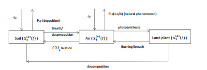
    [13] M. Fu, L. Tian, G. Dong, et al. Modeling on Regional Atmosphere-Soil-Land plant Carbon Cycle Dynamic System, Sustainability, 8 (2016), 303.
    [14] P. Arena, R. Caponetto, L. Fortuna, et al. Nonlinear noninteger order circuits and systems: An Introduction, World Scientific Series on Nonlinear Science, Series A: Monographs and Treatises, World Sci. Publishing, River Edge, NJ, 2000.
    [15] S. Song, B. Zhang, X. Song, et al. Neuro-fuzzy-based adaptive dynamic surface control for fractional-order nonlinear strict-feedback systems with input constraint, IEEE Transactions on Systems, Man, and Cybernetics: Systems, 2019.
    [16] X. Wang, Z. Wang, X. Zhu, et al. Stability and Hopf Bifurcation of Fractional-Order ComplexValued Neural Networks With Time-Delay, IEEE Access, 7 (2019), 158798-158807. doi: 10.1109/ACCESS.2019.2950276
    [17] S. Song, J. H. Park, B. Zhang, et al. Adaptive hybrid fuzzy output feedback control for fractionalorder nonlinear systems with time-varying delays and input saturation, Appl. Math. Comput., 364 (2020), 124662.
    [18] R. Hilfer, Applications of fractional calculus in physics, World Sci. Publishing, River Edge, NJ, 2000.
    [19] E. Ahmed and A. S. Elgazzar, On fractional order differential equations model for nonlocal epidemics, Physica A, 379 (2007), 607-614. doi: 10.1016/j.physa.2007.01.010
    [20] E. S. A. Shahri, A. Alfi and J. A. T. Machado, Stabilization of fractional-order systems subject to saturation element using fractional dynamic output feedback sliding mode control, J. Comput. Nonlinear Dyn., 12 (2017), 31014.
    [21] A. M. A. El-Sayed, A. E. M. El-Mesiry, H. A. A. El-Saka, On the fractional-order logistic equation, Appl. Math. Lett., 20 (2007), 817-823. doi: 10.1016/j.aml.2006.08.013
    [22] W. M. Ahmad, R. El-Khazali, Fractional-order dynamical models of love, Chaos Solitons Fractals, 33 (2007), 1367-1375. doi: 10.1016/j.chaos.2006.01.098
    [23] Z. J. Chen and W. J. Liu, Dynamical behavior of fractional-order energy-saving and emissionreduction system and its discretization, Nat. Resour. Model., 32 (2019), e12203.
    [24] W. J. Liu and K. W. Chen, Chaotic behavior in a new fractional-order love triangle system with competition, J. Appl. Anal. Comput., 5 (2015), 103-113.
    [25] Y. D. Liu and W. J. Liu, Chaotic behavior analysis and control of a toxin producing phytoplankton and zooplankton system based on linear feedback, Filomat, 32 (2018), 3779-3789. doi: 10.2298/FIL1811779L
    [26] D. Q. Chen and W. J. Liu, Chaotic behavior and its control in a fractional-order energy demandsupply system, J. Comput. Nonlin. Dyn., 11 (2016), 061010.
    [27] P. Song, H. Y. Zhao and X. B. Zhang, Dynamic analysis of a fractional order delayed predator-prey system with harvesting, Theor. Biosci., 135 (2016), 59-72. doi: 10.1007/s12064-016-0223-0
    [28] M. Caputo, Linear models of dissipation whose Q is almost frequency independent-II, Geophys. J. R. Astron. Soc., 13 (1967), 529-539. doi: 10.1111/j.1365-246X.1967.tb02303.x
    [29] A. E. Matouk, Chaos, feedback control and synchronization of a fractional-order modified autonomous Van der Pol-Duffing circuit, Commun. Nonlinear Sci., 16 (2011), 975-986. doi: 10.1016/j.cnsns.2010.04.027
    [30] D. Matignon, Stability results for fractional differential equations with applications to control Processing, CESA'96 IMACS Multiconference: Computational Engineering in Systems Applications, (1996), 963-968.
    [31] A. E. Matouk, Stability conditions, hyperchaos and control in a novel fractional order hyperchaotic system, Phys. Lett. A, 373 (2009), 2166-2173. doi: 10.1016/j.physleta.2009.04.032
    [32] A. E. Matouk, Dynamical behaviors, linear feedback control and synchronization of the fractional order Liu system, J. Nonlinear. Syst. Appl., 1 (2010), 135-140.
    [33] A. S. Hegazi, E. Ahemd and A. E. Matouk, The effect of fractional order on synchronization of two fractional order chaotic and hyperchaotic systems, J. Fract. Calc. Appl., 1 (2011), 1-15.
    [34] K. Diethelm, N. J. Ford and A. D. Freed, A predictor-corrector approach for the numerical solution of fractional differential equations, Nonlinear Dynam., 29 (2002), 3-22. doi: 10.1023/A:1016592219341
    [35] A. E. Matouk, A. A. Elsadany, E. Ahmed, et al. Dynamical behavior of fractional-order HastingsPowell food chain model and its discretization, Commun. Nonlinear Sci., 27 (2015), 153-167. doi: 10.1016/j.cnsns.2015.03.004
    [36] S. Elaydi, An introduction to difference equations, third edition, Undergraduate Texts in Mathematics, Springer, New York, 2005.
    [37] L. Edelstein-Keshet, Mathematical models in biology, The Random House/Birkhäuser Mathematics Series, Random House, New York, 1988.
    [38] J. Cao, S. Xue, J. Lin, et al. Nonlinear Dynamic Analysis of a Cracked Rotor-Bearing System With Fractional Order Damping, J. Comput. Nonlin. Dyn., 8 (2011), 031008.
  • This article has been cited by:

    1. Sameh Askar, Abdulrahman Al-khedhairi, Amr Elsonbaty, Abdelalim Elsadany, Chaotic Discrete Fractional-Order Food Chain Model and Hybrid Image Encryption Scheme Application, 2021, 13, 2073-8994, 161, 10.3390/sym13020161
    2. Tanfer Tanriverdi, Haci Mehmet Baskonus, Adnan Ahmad Mahmud, Kalsum Abdulrahman Muhamad, Explicit solution of fractional order atmosphere-soil-land plant carbon cycle system, 2021, 48, 1476945X, 100966, 10.1016/j.ecocom.2021.100966
    3. Mohammadreza Mahmoudi, Zohreh Eskandari, Fractional calculus in ecological systems: Bifurcation analysis and continuation techniques for discrete Lotka–Volterra models, 2024, 0170-4214, 10.1002/mma.10603
  • Reader Comments
  • © 2020 the Author(s), licensee AIMS Press. This is an open access article distributed under the terms of the Creative Commons Attribution License (http://creativecommons.org/licenses/by/4.0)
通讯作者: 陈斌, bchen63@163.com
  • 1. 

    沈阳化工大学材料科学与工程学院 沈阳 110142

  1. 本站搜索
  2. 百度学术搜索
  3. 万方数据库搜索
  4. CNKI搜索

Metrics

Article views(4263) PDF downloads(472) Cited by(3)

Figures and Tables

Figures(4)

Other Articles By Authors

/

DownLoad:  Full-Size Img  PowerPoint
Return
Return

Catalog