Research article Special Issues

Investigation and geotechnical characterization of Perniö clay, Finland

  • Understanding the behavior of soft sensitive clays is a key aspect of geotechnical design, especially in those regions where constructions are planned in marine clay areas. In Finland, one of the major geotechnical issues is the stability and deformation of the railway embankments located on soft soil deposits. The Tampere University of Technology (TUT) and the Finnish Transport Agency (FTA) have been carrying out a research project aiming to a better understanding of strength and deformation properties of Finnish soft clays. As a part of this project, a detailed site investigation was conducted at Perniö site in Western Finland. This paper presents the details of the geotechnical investigation, including field testing, sampling operations, and the laboratory testing program. In particular, an open drive tube sampler with 132 mm diameter, designed at TUT, was used to collect high quality samples. For comparison, samples were also taken using the conventional piston samplers and Sherbrooke Mini-block sampler. Field testing included piezocone, vane shear, and seismic piezocone. Laboratory testing consisted of index, consolidation, triaxial and simple shear tests. A comprehensive study of all these data is presented in a framework to describe Perniö soft clay.

    Citation: Bruno Di Buò, Marco D’Ignazio, Juha Selänpää, Markus Haikola, Tim Länsivaara, Marta Di Sante. Investigation and geotechnical characterization of Perniö clay, Finland[J]. AIMS Geosciences, 2019, 5(3): 591-616. doi: 10.3934/geosci.2019.3.591

    Related Papers:

    [1] Ke Bi, Yue Tan, Ke Cheng, Qingfang Chen, Yuanquan Wang . Sequential shape similarity for active contour based left ventricle segmentation in cardiac cine MR image. Mathematical Biosciences and Engineering, 2022, 19(2): 1591-1608. doi: 10.3934/mbe.2022074
    [2] Haiyan Song, Cuihong Liu, Shengnan Li, Peixiao Zhang . TS-GCN: A novel tumor segmentation method integrating transformer and GCN. Mathematical Biosciences and Engineering, 2023, 20(10): 18173-18190. doi: 10.3934/mbe.2023807
    [3] Jun Gao, Qian Jiang, Bo Zhou, Daozheng Chen . Convolutional neural networks for computer-aided detection or diagnosis in medical image analysis: An overview. Mathematical Biosciences and Engineering, 2019, 16(6): 6536-6561. doi: 10.3934/mbe.2019326
    [4] Jian Xu, Qian Shao, Ruo Chen, Rongrong Xuan, Haibing Mei, Yutao Wang . A dual-path neural network fusing dual-sequence magnetic resonance image features for detection of placenta accrete spectrum (PAS) disorder. Mathematical Biosciences and Engineering, 2022, 19(6): 5564-5575. doi: 10.3934/mbe.2022260
    [5] Qian Wu, Yuyao Pei, Zihao Cheng, Xiaopeng Hu, Changqing Wang . SDS-Net: A lightweight 3D convolutional neural network with multi-branch attention for multimodal brain tumor accurate segmentation. Mathematical Biosciences and Engineering, 2023, 20(9): 17384-17406. doi: 10.3934/mbe.2023773
    [6] Xi Lu, Zejun You, Miaomiao Sun, Jing Wu, Zhihong Zhang . Breast cancer mitotic cell detection using cascade convolutional neural network with U-Net. Mathematical Biosciences and Engineering, 2021, 18(1): 673-695. doi: 10.3934/mbe.2021036
    [7] Xiao Zou, Jintao Zhai, Shengyou Qian, Ang Li, Feng Tian, Xiaofei Cao, Runmin Wang . Improved breast ultrasound tumor classification using dual-input CNN with GAP-guided attention loss. Mathematical Biosciences and Engineering, 2023, 20(8): 15244-15264. doi: 10.3934/mbe.2023682
    [8] M Nisha, T Kannan, K Sivasankari . A semi-supervised deep neuro-fuzzy iterative learning system for automatic segmentation of hippocampus brain MRI. Mathematical Biosciences and Engineering, 2024, 21(12): 7830-7853. doi: 10.3934/mbe.2024344
    [9] Yufeng Li, Chengcheng Liu, Weiping Zhao, Yufeng Huang . Multi-spectral remote sensing images feature coverage classification based on improved convolutional neural network. Mathematical Biosciences and Engineering, 2020, 17(5): 4443-4456. doi: 10.3934/mbe.2020245
    [10] Vasileios E. Papageorgiou, Georgios Petmezas, Pantelis Dogoulis, Maxime Cordy, Nicos Maglaveras . Uncertainty CNNs: A path to enhanced medical image classification performance. Mathematical Biosciences and Engineering, 2025, 22(3): 528-553. doi: 10.3934/mbe.2025020
  • Understanding the behavior of soft sensitive clays is a key aspect of geotechnical design, especially in those regions where constructions are planned in marine clay areas. In Finland, one of the major geotechnical issues is the stability and deformation of the railway embankments located on soft soil deposits. The Tampere University of Technology (TUT) and the Finnish Transport Agency (FTA) have been carrying out a research project aiming to a better understanding of strength and deformation properties of Finnish soft clays. As a part of this project, a detailed site investigation was conducted at Perniö site in Western Finland. This paper presents the details of the geotechnical investigation, including field testing, sampling operations, and the laboratory testing program. In particular, an open drive tube sampler with 132 mm diameter, designed at TUT, was used to collect high quality samples. For comparison, samples were also taken using the conventional piston samplers and Sherbrooke Mini-block sampler. Field testing included piezocone, vane shear, and seismic piezocone. Laboratory testing consisted of index, consolidation, triaxial and simple shear tests. A comprehensive study of all these data is presented in a framework to describe Perniö soft clay.


    The chemostat is a laboratory bio-reactor used for the continuous culture of microorganism (Figure 1). The apparatus is of both ecological and mathematical interest since it can be used to represent a lot of microorganism systems, such as the simple lake and the waste-water treatment, and plays an important role in micrology and population [8,9,30].

    Figure 1.  The sketch map of chemostat and turbidostat: 1. Reservoir of sterile medium; 2. Valve controlling flowofmedium; 3. Outletforspentmedium; 4. Photocell; 5. Lightsource.

    Recently, a large of research devoted to modifying the chemostat for higher economical values by controlling the dilution rate of the chemostat. The chemostat with the feedback control of the dilution rate is established, which is referred to as turbidostat by biologists [14] (Figure 1). In the turbidostat, the optical sensor measures the concentration of the microorganism and the signal feedback control the dilution rate. For example, Flegr [5] analyzed the coexistence of two species in the turbidostat by numerical analysis, and later Leenheer and Smith [13] also demonstrated results of Flegr by theoretical analysis. They showed that a turbidostat with monotone response functions permits a unique coexistence equilibrium and if it is locally asymptotically stable then it is globally attracting. Furthermore, they also obtained that coexistence is not achievable in the turbidostat with more than two competing organisms. Li [14] established a mathematical model of competition in a turbidostat for an inhibitory nutrient and achieved the stability of the equilibrium and the existence of limit cycles. Li and Chen [16] studied a mathematical model of the turbidostat with impulsive state feedback control and obtained the existence and the stability of periodic solutions of order one.

    The uptake function in the model of microorganism continuous culture is the growth rate of the microorganism including many forms, such as, Monod [19], Moser [20] and Contois [4]. The most classical and common uptake function is Monod one, which is the function of concentration of microorganism and the constant half saturation term. However, Contois [4] presented experimental results to show that it is not necessarily a constant. Thus, the uptake function of Contois was introduced, which depends on the ratio substrate to microorganism. Jost [24] explored the relation of the Contois growth rate in microbiology and the ratio-dependent functional response in population ecology introduced by Arditi and Ginzburg [1]. As such, many researchers also call it ratio-dependent growth rate just as in population ecology [10,11,17,34]. Especially, Hu et al. [11] investigated the existence and the stability of the periodic solution of order one for the turbidostat system with ratio-dependent growth rate and impulsive state feedback control. The Contois model gave predictions that were in excellent agreement with experiment measurement. Especially, the Contois model was found to accurately describe the processing of industrial wastewaters. Nelson investigated a series of chemostat models with Contois growth rate. For example, Nelson and Sidhu [21] investigated the Hopf bifurcation and degenerate Hopf bifurcation of the chemostat model with Contois growth rate and the variable yield. Alqahtani et al. [22] studied the chemostat model with variable yield and contois growth kinetics with substrate inhibition and showed the Hopf bifurcation, degenerate Hopf bifurcation and Bogdanov-Takens bifurcation.

    Researchers recognized that time delays are natural in the ecological systems [12,27,29]. Smith and Waltman [30] showed that there are two obvious sources of delays in the cultivation of microorganism, one of which is the possibility that the microorganism stores the nutrient. Caperon [3] first introduced the delay into the chemostat model by some experiments. Bush and Cook [2] corrected Caperon's model and established a chemostat model with delay in the growth rate of microorganism. The time delays yield some complex impacts to the chemostat model and biologists gave the reasonable explanations for the observations and experimental datas by investigating the chemostat model with delays [18,15,23,26,31]. For example, Li et al. [15] considered the global dynamics of the chemostat model with two populations of microorganisms competing for two perfectly complementary nutrients when distributed delays are involved. Ruan and Wolkowicz [26] studied the existence and the stability of the Hopf bifurcation of the chemostat model with a distributed delay and found that the periodic solutions become unstable if the dilution rate is increased. Wang and Wolkowicz [31] analyzed the local stability of the equilibria and the globally asymptotical stability of the single species survival equilibrium when n species compete in the chemostat with time delay for a single resource, hence the competitive exclusion principle holds. Yao et al. [32] discussed the delayed turbidostat model with Monod growth rate and obtained the phenomenon of oscillation. In the turbidostat, additional factor causing delay is due to the process that the sensor controls the dilution, for example, Tagashira and Hara [28] and Yuan et al. [33] considered the turbidostat models of the dilution rate with delayed feedback control.

    Li and Xu [17] investigated the following chemostat system with Contois growth rate and time delay

    {dS(t)dt=d(S0S(t))1α+βS(t)mS(t)x(t)ax(t)+S(t),dx(t)dt=x(t){mS(tτ)ax(tτ)+S(tτ)d}, (1.1)

    where S(t) and x(t) present the concentration of substrate and the concentration of microorganism at time t , respectively, S0>0 stands for the input concentration of the nutrient, α+βS(t) (α>0,β>0) is variable yield, m>0 and a>0 are growth parameters of the microorganism, τ>0 is the time delay of the growth response of the microorganism, and d>0 presents the flow volume. They considered the local and global stability of the equilibria and Hopf bifurcation.

    In this paper, motivated by the works of Bush and Cook ([2]), Contois ([4]) and Li and Xu ([17]), one focuses on the dynamics of a turbidostat model with Contois growth rate and time delay which follows as

    {dS(t)dt=(d+kx(t))(S0S(t))1γmS(t)x(t)ax(t)+S(t),dx(t)dt=x(t){mS(tτ)ax(tτ)+S(tτ)dkx(t)}, (1.2)

    where S(t) , x(t) and parameters S0 , m , a , τ are defined as in (1.1), γ>0 is yield constant and d+kx(t) (d>0,k>0) presents the dilution rate of the turbidostat.

    The aim of this paper is to investigate the qualitative properties of system (1.2) including the stability of the equilibria and the bifurcations. The outline of this paper is as follows. In Section 2, I analyze the existence and local stability of the equilibria, and the transcritical bifurcation at the boundary equilibrium and the Hopf bifurcation at the positive equilibrium. In Section 3 mostly focuses on the stability and type of the bifurcating periodic solutions induced by Hopf bifurcation to system (1.2). I in Section 4 further illustrate our main results by numerical simulations.

    In this section, we investigate the existence and stability of the equilibria and the bifurcations at equilibria including the transcritical bifurcation and Hopf bifurcation of system (1.2).

    It is convenient to introduce dimensionless variables. In particular, we set

    S=˜SS0,x=˜xγS0,k=d˜kγS0,a=˜aγ,m=d˜m,t=˜td.

    System (1.2) becomes

    {dS(t)dt=(1+kx(t))(1S(t))mS(t)x(t)ax(t)+S(t),dx(t)dt=x(t)(mS(tτ)ax(tτ)+S(tτ)1kx(t)), (2.1)

    where we still denote ˜S,˜x,˜k,˜a,˜m,˜t with S,x,k,a,m,t , respectively. First of all, we discuss the existence of the equilibria of system (2.1) and have the following result.

    Lemma 2.1. System (2.1) always has a boundary equilibrium E0:(1,0) ; If m>1 , then system (2.1) has a unique positive equilibrium E1:(S,x) , where S=1+km+k when a=1 ,

    S=(2ak+ak+m1)+(2ak+ak+m1)2+4ak(1a)(1+k)2k(1a),

    when a1 and x=1S .

    Proof. From the right part of system (2.1), we can obtain the boundary equilibrium easily, which we denote as E0:(1,0) . In order to get the positive equilibrium, we need to discuss the roots of the equation mSa+(1a)S1k(1S)=0 on the interval (0,1) . We define

    f(S):=(1a)kS2+(2ak+ak+m1)Sa(1+k). (2.2)

    Therefore, we just need to discuss the zeros of the function f(S) on the interval (0,1) , which need to be discussed in the following three cases.

    (ⅰ). If a=1 , then we have f(S)=(k+m)S1K and f(S) has a zero S=1+km+k on the interval (0,1) when m>1 , and f(S) has no zero on the interval (0,1) when m1 . Thus, we obtain S=1+km+k when a=1 and m>1 .

    (ⅱ). If 0<a<1 , then f(S) is a quadratic function of S . Since the coefficient of quadratic term k(1a)>0 and f(0)=a(1+k)<0 , f(S)=0 has two roots

    S1:=(2ak+ak+m1)(2ak+ak+m1)2+4ak(1a)(1+k)2k(1a),S2:=(2ak+ak+m1)+(2ak+ak+m1)2+4ak(1a)(1+k)2k(1a), (2.3)

    and it is obvious that S1<0,S2>0 . By simplifying the inequality S2<1 , we can get that S2<1 if and only if m>1 . Thus, we have S=S2 when 0<a<1 and m>1 .

    (ⅲ). If a>1 , then f(S) still is a quadratic function of S with the coefficient of quadratic term k(1a)<0 and f(0)=a(1+k)<0 . The discriminant of f(S) is

    Δ:=a2+2(2kmk+m1)a+(km+1)2.

    We can take Δ as the function of a . Therefore, the discriminant of Δ is ˜Δ:=km(m1)(1+k) . For this case we need further discussion in the following three cases.

    (a). If m=1 , then ˜Δ=0 and the double root of Δ=0 is k . Therefore, Δ>0 holds when a>1 . We have f(S)=0 has two roots S1=a(1+k)k(a1)>1 and S2=1 . Thus, f(S) has no zero on the interval (0,1) when a>1 and m=1 .

    (b). If m<1 , then ˜Δ<0 , which implies Δ>0 . We have f(S) has two roots S1 and S2 presented in (2.3) and S2<S1 . By simplifying S2>1 , we can get that S2>1 if and only if m<1 . Thus, f(S) has no zero on the interval (0,1) when a>1 and m<1 .

    (c). If m>1 , then ˜Δ>0 . Since 4km2k+2m2>0 and (km+1)20 , the two roots of Δ=0 denoted by a1 and a2 satisfy a1<a20 . Therefore, Δ>0 holds when a>1 and m>1 . We obtain f(S) has two roots presented in (2.3) and S1>S2 . Further, we can get 0<S2<1 if and only if m>1 and a>1 . Suppose that S1<1 , then we get m>1 , which is a contradiction. Thus, we have S=S2 when a>1 and m>1 .

    This completes the proof.

    From the above analysis we have the existence of equilibria of system (2.1). In the following, we consider qualitative properties of system (2.1) including stability of the equilibria and the bifurcations. We discuss system (2.1) in two cases: (ⅰ) τ=0 and (ⅱ) τ>0 .

    Case (ⅰ): τ=0 , i.e. there is no time delay in system (2.1), then system (2.1) becomes

    {dS(t)dt=(1+kx(t))(1S(t))mS(t)x(t)ax(t)+S(t),dx(t)dt=x(t)(mS(t)ax(t)+S(t)1kx(t)). (2.4)

    We first investigate the stability of the equilibria E0 and E1 and have the following result.

    Theorem 2.2. If m<1 , then E0 is a stable node; If m>1 , then E0 is a saddle and E1 is a stable node; If m=1 , then E0 is a saddle-node.

    Proof. The Jacobian matrix at E0 is

    J0:=(1m0m1).

    The determinant, trace and discriminant are respectively

    D0:=1m,T0:=m2,Δ0:=T204D0=m2>0.

    If m<1 , then D0>0 and T0<0 . Thus, E0 is a stable node. If m>1 , then D0<0 . Thus, E0 is a saddle. If m=1 , then D0=0 and T0=1 . This is the degenerate case, which needs further discussion.

    Translating the equilibrium E0 to the origin by ˜S=S1 , system (2.4) becomes the following system

    {dS(t)dt=S(t)(1+kx(t))(S(t)+1)x(t)ax(t)+S(t)+1,dx(t)dt=x(t)(S(t)+1ax(t)+S(t)+11kx(t)), (2.5)

    where we still use S to present ˜S . Using the linear transformation u=x , v=S+x and time-rescaling t1=t to normalize the linear part of system (2.5), we can change system (2.5) into the following

    {dudt=(a+k)u2+a(1a)u3au2v+:=Φ(u,v),dvdt=v+kuv:=Ψ(u,v), (2.6)

    where we still denote t1 as t . By the implicit function theorem, there is a unique function v=ϕ(u) such that Ψ(u,v)=0 . We can obtain v=ϕ(u)=0 by solving Ψ(u,v)=0 . Substituting v=0 into Φ(u,v)=0 , we get

    Φ(u,v)=(a+k)u2+a(1a)u3+.

    Thus E0 is a saddle-node when m=1 by Theorem 7.1 in Zhang et al. ([35]). Moreover, the parabolic sector of the saddle-node lies on the right-hand plane in the (u,v) -coordinates and the two hyperbolic sectors lie on the left-hand plane since a+k>0 .

    We continue to prove the properties of E1 .

    The Jacobian matrix at E1 is

    J1:=(1kxma(x)2(ax+S)2kxm(S)2(ax+S)2ma(x)2(ax+S)212kx+m(S)2(ax+S)2).

    The determinant, trace and discriminant of J1 are respectively

    D1:=(1+kx){maSx+kx(ax+S)2+max(ax+S)2}>0,T1:=23kx+m(S)2(ax+S)2ma(x)2(ax+S)2T1:={1+2k+maSx(ax+S)2+ma(x)2(ax+S)2}<0,Δ1:=T214D1={kx+m(S)2(ax+S)2ma(x)2(ax+S)2}20.

    Thus, E1 is a stable node if it exists.

    We complete the proof.

    It is indicated in Lemma 2.1 that system (2.4) has either exact one equilibrium E0 when m1 or exact two equilibria E0 and E1 when m>1 . In the following we reduce the system to a 1-dimensional system on a center manifold and display the mechanism for E1 to arise.

    Theorem 2.3. System (2.4) experiences a transcritical bifurcation at E0 when m=1 .

    Proof. Let ε=m1 and translate the equilibrium E0 to the origin by ˜S=S1 , system (2.4) becomes the following system

    {dSdt=(1+kx)S(1+ε)(S+1)ax+S+1x,dxdt=x{(1+ε)(S+1)ax+S+11kx}, (2.7)

    where we still denote ˜S as S .

    Applying the transformation S=u+v and x=u to diagonalize the linear part of system (2.7), we can change system (2.7) into the suspended system

    {dudt=εu(a+k)u2aεu2+au2v+a(a1)u3+,dvdt=vkuv,dεdt=0. (2.8)

    By the center manifold theory, system (2.8}) has a two-dimensional center manifold Wc:v=h(u,ε) near O , which is tangent to the plane v=0 at O in the (u,v,ε) -space. In order to obtain the second-order approximation of function h , we set

    v=h(u,ε)=a1u2+b1uε+c1ε2+o(|u,ε|2). (2.9)

    Substituting (2.9) into the equality ˙v=hu˙u and comparing the coefficient of u2 , ε2 and uε , we have a1=b1=c1=0 . Hence the center manifold is v=o(|u,ε|2) and the restricted system of (2.8}) on the center manifold (2.9) is

    dudt=εu(a+k+aε)u2+a(a1)u3+. (2.10)

    The expression (2.10) shows that a transcritical bifurcation occurs at E0 as ε varies through the bifurcation value ε=0 ([6]). More concretely, when ε<0 , E0 is stable and the other equilibrium appears on the negative u -axis; when ε=0 , the two equilibria coincide at E0 , which is a saddle-node; when ε>0 , E0 remains an equilibrium but is unstable while a stable equilibrium E1 arises.

    We complete the proof.

    Case (ⅱ): τ>0 .

    In this case we will investigate the effect of time delay on the system. The time delay can cause the loss of stability of E1 and can induce periodic solutions. Note that if m>1 , then system (2.1) has a unique positive equilibrium E1 . To further consider the local stability of E1 and the Hopf bifurcations induced by the delay, we set ˜x(t)=x(t)x,˜S(t)=S(t)S and still denote ˜x,˜S as x,S . Then system (2.1) can be changed into the following system

    {dS(t)dt=a11S(t)+a12x(t)+a13S2(t)+a14x2(t)+a15S(t)x(t)dS(t)dt=+a16x3(t)+a17S(t)x2(t)+a18S2(t)x(t)+a19S3(t)+,dx(t)dt=b11S(tτ)+b12x(t)+b13x(tτ)+b14S2(tτ)+b15x2(t)dx(t)dt=+b16x2(tτ)+b17S(tτ)x(t)+b18x(t)x(tτ)dx(t)dt=+b19S(tτ)x(tτ)+b20x(t)x2(tτ)+b21x3(tτ)dx(t)dt=+b22x(t)x(tτ)S(tτ)+b23S(tτ)x2(tτ)dx(t)dt=+b24S2(tτ)x(t)+b25x(tτ)S2(tτ)+b26S3(tτ)+, (2.11)

    where

    a11=1kxma(x)2(ax+S)2,a12=kxm(S)2(ax+S)2,a13=ma(x)2(ax+S)3,a14=ma(S)2(ax+S)3,a15=k2maSx(ax+S)3,a16=ma2(S)2(ax+S)4,a17=maS(2axS)(ax+S)4,a18=max(ax2S)(ax+S)4,a19=ma(x)2(ax+S)4,b11=ma(x)2(ax+S)2,b12=12kx+mSax+S,b13=maSx(ax+S)2,b14=ma(x)2(ax+S)3,b15=k,b16=ma2Sx(ax+S)2,b17=max(ax+S)2,b18=maS(ax+S)2,b19=max(axS)(ax+S)3,b20=ma2S(ax+S)3,b21=ma3Sx(ax+S)4,b22=ma(axS)(ax+S)3,b23=ma2x(ax2S)(ax+S)4,b24=max(ax+S)3,b25=max(2axS)(ax+S)4,b26=ma(x)2(ax+S)4.

    The following characteristic equation can be achieved from the linear system of system (2.11)

    λ2(a11+b12)λ+eλτ(b13λ+a11b13a12b11)+a11b12=0. (2.12)

    To investigate the stability of the equilibrium E1 and Hopf bifurcation of (2.1), we must study the distribution of the roots of (2.12).

    Lemma 2.4. If a11b12+a12b11a11b13<0 , then ±iw0(w0>0) are the eigenvalues of (2.12) when τ=τj . The values of w0 and τj can be presented as follows

    w0=2a11b12+b213(a11+b12)2+{2a11b12b213+(a11+b12)2}24{a211b212(a11b13a12b11)2}2,τj=1w0{arccos((w20a11b12)(a11b13a12b11)b13(a11+b12)w20(a11b13a12b11)2+b213w20)+2jπ},j=0,1,2.

    Proof. If λ=iw (w>0) is a root of (2.12), then we have

    w2iw(a11+b12)+(coswτisinwτ)(ib13w+a11b13a12b11)+a11b12=0.

    Separating the real and imaginary parts, we obtain

    (a11b13a12b11)coswτb13wsinwτ=w2a11b12,(a11b13a12b11)sinwτ+b13wcoswτ=w(a11+b12), (2.13)

    which implies the following equation

    w4+{2a11b12+(a11+b12)2b213}w2+a211b212(a11b13a12b11)2=0.

    Denote

    h(w):=w4+(a211+b212b213)w2+a211b212(a11b13a12b11)2.

    Since

    a11b12+a11b13a12b11=(1+kx){kx+maSx(ax+S)2}+m2aS(x)2(ax+S)(ax+S)4>0

    and the condition a11b12+a12b11a11b13<0 , we have the constant term of h(w) is negative. In addition, we can obtain the coefficient of quadratic term of h(w) is positive. In fact,

    a211+b212b213={1+kx+ma(x)2(ax+S)2}2+(1+2kxmSax+S)2(maSx)2(ax+S)4a211+b212b213={mSax+S+ma(x)2(ax+S)2}2+(kx)2(maSx)2(ax+S)4a211+b212b213=m2{(S)2+a(x)2}2+2m2aSx{(S)2+a(x)2}(ax+S)4+(kx)2>0.

    Thus, h(w) has a unique positive real root

    w0=22{2a11b12+b213(a11+b12)2w0+(2a11b12b213+(a11+b12)2)24(a211b212(a11b13a12b11)2)}12. (2.14)

    Substituting w0 into (2.13), we conclude that

    (2.15)

    Hence, (2.12) has a pair of purely imaginary roots ±iw0 as τ=τj, j=0,1,2 .

    This completes the proof.

    Let λ(τ)=α(τ)+iβ(τ) denote the root of (2.12) near τ=τj satisfying α(τj)=0 and β(τj)=w0 . Then we have the following transversality condition.

    Lemma 2.5. The following transversality condition holds

    dRe(λ(τj))dτ>0,j=0,1,2.

    Proof. Differentiating (2.12) with respect to τ yields that

    (dλdτ)1=(2λa11b12)eλτb13λ(b13λ+a11b13a12b11)τλ.

    Thus,

    Re{(dλ(τj)dτ)1}=Re{(2iw0a11b12)(cosw0τ+isinw0τ)b13w20b13+iw0(a11b13a12b11)}Re{(dλ(τj)dτ)1}=h(w0)2w30b213+2w0(a11b13a12b11)2.

    Since h(w) is a quartic function of w and the leading coefficient of which is positive, furthermore, from the analysis of Lemma 2.4, we obtain that the four roots of equation h(w)=0 are a pair of conjugate complex roots, a negative real root and a positive real root w0 , respectively. Hence h(w) is monotonically increasing at w0 , i.e., h(w0)>0 , which implies h(w0)/{2w30b213+2w0(a11b13a12b11)2}>0 . Thus, we have

    sign{Re(dλ(τj)dτ)}=sign{Re(dλ(τj)dτ)1}=1.

    The proof is completed.

    Now we have the following result about the distribution of the roots of the exponential polynomial (2.12) by Corollary 2.4 in [25].

    Lemma 2.6. Suppose that w0 and τj (j=0,1,2) are defined by (2.14) and (2.15), respectively. We have the following results

    (i ) If a11b12+a12b11a11b130 , then all the roots of (2.12) have negative real parts for all τ>0 .

    (ii ) If a11b12+a12b11a11b13<0 and τ=τj , then (2.12) has a pair of simple imaginary roots ±iw0 . Furthermore, if τ[0,τ0) , then all the roots of (2.12) have negative real parts; if τ(τj,τj+1),j=0,1,2 , then (2.12) has at least one root with positive real parts.

    From Lemma 2.4, Lemma 2.5, Lemma 2.6 and the Hopf bifurcation theorem, we have the following result of E1 .

    Theorem 2.7. For system (2.1), we have

    (i ) if a11b12+a12b11a11b130 , then the unique positive equilibrium E1 is asymptotically stable for all τ0 .

    (ii ) if a11b12+a12b11a11b13<0 , then the equilibrium E1 is asymptotically stable for τ[0,τ0) and unstable for τ>τ0 . Hopf bifurcation occurs when τ=τj,j=0,1,2 .

    In this section, we consider the direction and stability of the bifurcating periodic solutions of system (2.1) induced by the Hopf bifurcation by using the normal form theory and the center manifold theorem by Hassard et al. ([7]). We compute (see Appendix for details of the computation)

    g(z,ˉz)=g20z22+g11zˉz+g02ˉz22+g21z2ˉz2+,

    where the first four coefficients g20 , g11 , g02 and g21 that we need for determining the properties of the Hopf bifurcation are of the following forms

    g20=2τjˉD{a14q21+a15q1+a13+ˉq1(b15q21+(b18q21+b17q1)eiw0τj+(b16q21g21=+b19q1+b14)e2iw0τj)},g11=τjˉD{a15q1+a15ˉq1+2a13+2a14ˉq1q1+ˉq1(2b14+b19q1+b19ˉq1+2b15ˉq1q1g21=+2b16ˉq1q1+(b17ˉq1+b18q1ˉq1)eiw0τj+(b17q1+b18ˉq1q1)eiw0τj)},g02=2τjˉD{a13+a14ˉq21+a15ˉq1+ˉq1(b15ˉq21+(b16ˉq21+b19ˉq1+b14)e2iw0τj+(b18ˉq21g21=+b17ˉq1)eiw0τj)},g21=τjˉD{3a16q21ˉq1+a17q21+2a17q1ˉq1+2a18q1+a18ˉq1+3a19+(12a15g21=+a14ˉq1)W(2)20(0)+(a15+2a14q1)W(2)11(0)+(a15q1+2a13)W(1)11(0)+(12a15ˉq1g21=+a13)W(1)20(0)+ˉq1(2b24q1+(b22q1+b22ˉq1)q1+(3b26+2b23ˉq1q1+3b21ˉq1q21g21=+b23q21+b25ˉq1+2b25q1)eiw0τj+(b24ˉq1+b20q21ˉq1+b22q1ˉq1)e2iw0τjg21=+2b20ˉq1q21+((b19q1+2b14)eiw0τj+b17q1)W(1)11(1)+((12b19ˉq1+b14)eiw0τjg21=+12b17ˉq1)W(1)20(1)+((b18q1+b17)eiw0τj+2b15q1)W(2)11(0)+(12(b18ˉq1g21=+b17)eiw0τj+b15ˉq1)W(2)20(0)+((2b16q1+b19)eiw0τj+b18q1)W(2)11(1)g21=+((b16ˉq1+12b19)eiw0τj+12b18ˉq1)W(2)20(1))},

    in which the terms W(1)11(0) , W(2)11(0) , W(1)11(1) , W(2)11(1) , W(1)20(0) , W(2)20(0) , W(1)20(1) , W(2)20(1) , q1 , q1 and ˉD are calculated in Appendix.

    Now using the four coefficients we obtain the values of the parameters μ2 , β2 and T2

    c1(0)=i2w0τj(g11g202|g11|213|g02|2)+g212,μ2=Re(c1(0))Re(λ(τj)),β2=2Re(c1(0)),T2=Im(c1(0))+μ2Im(λ(τj))w0τj.

    Thus, using the quantities above, the properties of the Hopf bifurcation are determined by the following theorem.

    Theorem 3.1. The properties of the Hopf bifurcation are determined by the parameters μ2 , β2 and T2 , where μ2 determines the direction of the Hopf bifurcation: if μ2>0 (<0) , then the Hopf bifurcation is supercritical (subcritical); β2 determines the stability of the bifurcating periodic solutions: if β2<0 (>0) , the bifurcating periodic solutions are stable (unstable); and T2 determines the period of the bifurcating periodic solutions: if T2>0 (<0) , the period increases (decreases).

    We discussed a turbidostat system with Contois growth rate and time delay in this paper. We investigated the qualitative properties of system (1.2) including the existence and the stability of the equilibria and the bifurcations. In the case of no time delay, the boundary equilibrium E0 is globally asymptotically stable if it is the unique equilibrium, and the positive equilibrium E1 arising from a transcritical bifurcation is globally asymptotically stable if it exists. In the case of system with delay, the stability of E1 is changed and the Hopf bifurcation occurs by choosing the delay as the bifurcation parameter. Furthermore, the stability and direction of the bifurcating periodic solutions are discussed by using the normal form and center manifold theorem. More concretely, when the delay is greater than the critical value τ0 , the positive equilibrium E1 loses its stability and the stable periodic solution appears. The qualitative analysis and theoretical results show that the delay can change the topological structures of the system and produces more complicated dynamic behaviors.

    We next offer an example to illustrate the feasibility of our results. When system (2.1) without delay, i.e. τ=0 , we set a=1 and k=0.6 , the system has the unique equilibrium E0 , which is a stable node as m=0.5 ; the system has a saddle E0 and a stable node E1=(0.76,0.24) as m=1.5 ; the system has the unique equilibrium E0 , which is a saddle-node as m=1 (Figure 2). However, when m=1.5 , a=1 and k=0.6 , by choosing the time delay τ as the bifurcation parameter, we obtained the critical value of bifurcation τ07 . Thus, the positive equilibrium E1 is asymptotically stable when τ=6<τ0 , which is supported by Figure 3. The positive equilibrium E1 is unstable and a stable bifurcating periodic solution occurs from E1 when τ=8>τ0 , which can be seen clearly in Figure 4. According to (4.10) we can compute

    g204.259.16i,g110.21+1.3i,g0211.790.01i,g2147.165.86i.
    Figure 2.  (a) When m=0.5 , a=1 and k=0.6 , E0 is the unique equilibrium and is a stable node; (b) When m=1.5 , a=1 and k=0.6 , E0 is a saddle and E1=(0.76,0.24) is a stable node; (c) When m=1 , a=1 and k=0.6 , E0 is the unique equilibrium and is a saddle-node.
    Figure 3.  The positive equilibrium E1=(0.76,0.24) of system (2.1) is asymptotically stable when m=1.5 , a=1 , k=0.6 and τ=6<τ07 . Here (S(0),x(0))=(0.5,0.8).
    Figure 4.  The positive equilibrium E1=(0.76,0.24) of system (2.1) is unstable and a bifurcating stable periodic solution occurs from E1 when m=1.5 , a=1 , k=0.6 and τ=8>τ07 . Here (S(0),x(0))=(0.5,0.8).

    Further, we can get

    c1(0)21.7112.63i.

    Then, in accordance with (4.22), we can obtain

    μ22131.70>0,β243.42<0,T238.7>0.

    Therefore, when τ=8 , μ2>0 and β2<0 , then the Hopf bifurcation for system (2.1) is supercritical and the stable bifurcating periodic solutions occur from the positive equilibrium E1 . From Figure 3 and Figure 4, we can find that the dynamics of system (2.1) change when τ locates near τ0 . The bifurcation diagram of xτ is presented in Figure 5, from which we find that even for parameter values not chosen, the stable periodic solutions occur in a large region of time delay.

    Figure 5.  The bifurcation diagram of xτ with m=1.5 , a=1 , k=0.6 and (S(0),x(0))=(0.5,0.8).

    Remark 1. This is a remark about Figure 2. In fact, considering the biological background, the set Ω={(S,x):0S1,x0} is positively invariant with respect to system (2.4). Further, E0 is globally asymptotically stable with respect to Ω if m<1 ; E0 is globally attractive with respect to Ω if m=1 ; and E1 is globally asymptotically stable with respect to Ω if m>1 . These results can be proved easily by Liapunov-LaSalle invariant principle and Poincare-Bendixson Theorem respectively.

    The author is very grateful to the anonymous referees for their careful reading and valuable suggestions, which have notably improved the quality of this paper.

    All authors declare no conflicts of interest in this paper.

    We obtained in Section 2 that system (2.1) undergoes the Hopf bifurcation at the positive equilibrium E1 when τ=τj . In the following the properties of the Hopf bifurcation are determined. We first consider system (2.1) by the transformation ˜y1(t)=S(τt), ˜y2(t)=x(τt), τ=τj+μ and still denote ˜y1(t),˜y2(t) as y1(t),y2(t) . Then system (2.1) is equivalent to a functional differential equation defined in C=C([1,0],R2)

    ˙y(t)=Lμ(yt)+h(μ,yt), (4.1)

    where y(t)=(y1(t),y2(t))TR2 , and Lμ:CR2 and h:R×CR2 are given respectively by

    Lμφ=(τj+μ)(a11a120b12)(φ1(0)φ2(0))+(τj+μ)(00b11b13)(φ1(1)φ2(1))

    and

    h(μ,φ)=(τj+μ)(h1h2),

    where

    h1=a13φ21(0)+a14φ22(0)+a15φ1(0)φ2(0)+a16φ32(0)+a17φ1(0)φ22(0)h1=+a18φ21(0)φ2(0)+a19φ31(0)+,h2=b14φ21(1)+b15φ22(0)+b16φ22(1)+b17φ1(1)φ2(0)+b18φ2(0)φ2(1)h1=+b19φ1(1)φ2(1)+b20φ22(1)φ2(0)+b21φ32(1)h1=+b22φ2(0)φ2(1)φ1(1)+b23φ1(1)φ22(1)+b24φ21(1)φ2(0)h1=+b25φ21(1)φ2(1)+b26φ31(1)+,

    and φ=(φ1,φ2)TC.

    By the Riesz representation theorem, there exists a matrix whose components are bounded variation functions η(θ,μ) for θ[1,0] such that

    Lμφ=01dη(θ,μ)φ(θ)forφC.

    Indeed, we may choose

    η(θ,μ)=(τj+μ)(a11a120b12)δ(θ)(τj+μ)(00b11b13)δ(θ+1),

    where δ is the Dirac delta function.

    For φC1([1,0],R2) , we further define the operators A and B as

    A(μ)φ={dφ(θ)dθ,θ[1,0),01dη(θ,μ)φ(θ),θ=0,B(μ)φ={0,θ[1,0),h(μ,φ),θ=0.

    Then system (4.1) is equivalent to

    ˙yt=A(μ)yt+B(μ)yt, (4.2)

    where yt(θ)=y(t+θ) for θ[1,0] .

    For ψC1([0,1],(R2)) , we define A of A as

    Aψ={dψ(s)ds,s(0,1],01dηT(t,0)ψ(t),s=0.

    In order to normalize the eigenvectors of A and A , we define a bilinear inner product

    ψ(s),φ(θ)=ˉψT(0)φ(0)01θξ=0ˉψT(ξθ)dη(θ)φ(ξ)dξ, (4.3)

    where η(θ)=η(θ,0) .

    From the above discussion we assume q(θ) and q(s) are eigenvectors of A and A corresponding to iw0τj and iw0τj . Suppose that q(θ)=(1,q1)Teiw0τjθ is the eigenvector of A(0) corresponding to iw0τj , then Aq(0)=iw0τjq(0) . On the basis of the definitions of A(0) , Lμφ and η(θ,μ) , the following conclusion can be achieved

    τj(a11iw0a12b11eiw0τjb12b13eiw0τjiw0)(1q1)=(00).

    We can get

    q1=iw0a11a12. (4.4)

    Similarly, by the definition of A , we have

    τj(a11+iw0b11eiw0τja12b12+b13eiw0τj+iw0)(1q1)=(00)

    and

    q1=iw0a11b11eiw0τj. (4.5)

    We can then obtain the value of D by q,q=1 . Further it holds from (4.3) that

    q(s),q(θ)=ˉD(1,ˉq1)(1,q1)Tq(S),q(θ)=01θξ=0ˉD(1,ˉq1)eiw0τj(ξθ)dη(θ)(1,q1)Teiξw0τjdξq(S),q(θ)=ˉD{1+ˉq1q101(1,ˉq1)θeiθw0τjdη(θ)(1,q1)T}q(S),q(θ)=ˉD{1+ˉq1q1+τjeiw0τjˉq1(b11+b13q1)}.

    Hence

    D=11+q1ˉq1+τjeiw0τjq1(b11+b13ˉq1). (4.6)

    In the following part, we compute the coordinates describing center manifold C0 at μ=0 by using the theory in [7]. Define

    z(t)=q(s),yt(θ),W(t,θ)=yt(θ)2Re{z(t)q(θ)}. (4.7)

    Then on the center manifold C0 , we have

    W(t,θ)=W(z(t),ˉz(t),θ)=W20(θ)z22+W11(θ)zˉz+W02(θ)ˉz22+,

    where z and ˉz are local coordinates for center manifold C0 in the direction of q and ˉq . It is easy to see that W is real if yt is real. Thereby, we next only consider real solutions of (4.2). If ytC0 is the solution of (4.2), since μ=0 , which implies that

    ˙z(t)=<q,˙yt>=<q,A˙yt+B˙yt>=<Aq,˙yt>+<q,B˙yt>˙z(t)=iw0τjz+ˉq(0)h(0,W(z,ˉz,0)+2Re{zq(0)})˙z(t)def=iw0τjz+ˉq(0)h0(z,ˉz)=iw0τjz+g(z,ˉz),

    where

    g(z,ˉz)=ˉq(0)h0(z,ˉz)=g20z22+g11zˉz+g02ˉz22+g21z2ˉz2+. (4.8)

    In the following we need to compute the coefficients g20 , g11 , g02 and g21 . Note that yt(θ)=(y1t(θ),y2t(θ))T=W(t,θ)+zq(θ)+¯zq(θ) and q(θ)=(1,q1)Teiw0τjθ . It then follows that

    {y1t(0)=z+ˉz+W(1)20(0)z22+W(1)11(0)zˉz+W(1)02(0)ˉz22y1t(0)=+O(|(z,ˉz)|3),y2t(0)=q1z+¯q1ˉz+W(2)20(0)z22+W(2)11(0)zˉz+W(2)02(0)ˉz22y1t(0)=+O(|(z,ˉz)|3),y1t(1)=zeiw0τj+ˉzeiw0τj+W(1)20(1)z22+W(1)11(1)zˉzy1t(1)=+W(1)02(1)ˉz22+O(|(z,ˉz)|3),y2t(1)=q1zeiw0τj+ˉq1ˉzeiw0τj+W(2)20(1)z22+W(2)11(1)zˉzy1t(1)=+W(2)02(1)ˉz22+O(|(z,ˉz)|3). (4.9)

    It follows together with the definition h(μ,φ) that

    g(z,ˉz)=ˉq(0)h0(z,ˉz)g(z,ˉz)=τjˉD{a13φ21(0)+a14φ22(0)+a15φ1(0)φ2(0)+a16φ32(0)+a17φ1(0)φ22(0)g(z,ˉz)=+a18φ21(0)φ2(0)+a19φ31(0)++ˉq1(b14φ21(1)+b15φ22(0)g(z,ˉz)=+b16φ22(1)+b17φ1(1)φ2(0)+b18φ2(0)φ2(1)+b19φ1(1)φ2(1)g(z,ˉz)=+b20φ22(1)φ2(0)+b21φ32(1)+b22φ2(0)φ2(1)φ1(1)g(z,ˉz)=+b23φ1(1)φ22(1)+b24φ21(1)φ2(0)+b25φ21(1)φ2(1)g(z,ˉz)=+b26φ31(1)+)}.

    By substituting (4.9) into the above equation and comparing the coefficients with (4.8) we have

    {g20=2τjˉD{a14q21+a15q1+a13+ˉq1(b15q21+(b18q21+b17q1)eiw0τjg21=+(b16q21+b19q1+b14)e2iw0τj)},g11=τjˉD{a15q1+a15ˉq1+2a13+2a14ˉq1q1+ˉq1(2b14+b19q1+b19ˉq1g21=+2b15ˉq1q1+2b16ˉq1q1+(b17ˉq1+b18q1ˉq1)eiw0τjg21=+(b17q1+b18ˉq1q1)eiw0τj)},g02=2τjˉD{a13+a14ˉq21+a15ˉq1+ˉq1(b15ˉq21+(b16ˉq21+b19ˉq1g21=+b14)e2iw0τj+(b18ˉq21+b17ˉq1)eiw0τj)},g21=τjˉD{3a16q21ˉq1+a17q21+2a17q1ˉq1+2a18q1+a18ˉq1+3a19g21=+(12a15+a14ˉq1)W(2)20(0)+(a15+2a14q1)W(2)11(0)g21=+(a15q1+2a13)W(1)11(0)+(12a15ˉq1+a13)W(1)20(0)g21=+ˉq1(2b24q1+(b22q1+b22ˉq1)q1+(3b26+2b23ˉq1q1+3b21ˉq1q21g21=+b23q21+b25ˉq1+2b25q1)eiw0τj+(b24ˉq1+b20q21ˉq1g21=+b22q1ˉq1)e2iw0τj+2b20ˉq1q21+((b19q1+2b14)eiw0τjg21=+b17q1)W(1)11(1)+((12b19ˉq1+b14)eiw0τj+12b17ˉq1)W(1)20(1)g21=+((b18q1+b17)eiw0τj+2b15q1)W(2)11(0)+(12(b18ˉq1+b17)eiw0τjg21=+b15ˉq1)W(2)20(0)+((2b16q1+b19)eiw0τj+b18q1)W(2)11(1)g21=+((b16ˉq1+12b19)eiw0τj+12b18ˉq1)W(2)20(1))}. (4.10)

    In order to determine g21 we need to compute W20(θ) and W11(θ) . In the light of (4.2) and (4.7), we obtain

    ˙W=˙yt˙zq˙ˉzˉq˙W={AW2Re{ˉq(0)h0(z,ˉz)q(θ)},θ[1,0),AW2Re{ˉq(0)h0(z,ˉz)q(θ)}+h0(z,ˉz),θ=0,˙Wdef=AW+H(z,ˉz,θ), (4.11)

    where

    H(z,ˉz,θ)=H20(θ)z22+H11(θ)zˉz+H02(θ)ˉz22+H20(θ)z36+. (4.12)

    Expanding the previous series and comparing the coefficients, we obtain that

    {(A2iw0τjI)W20(θ)=H20(θ),AW11(θ)=H11(θ),. (4.13)

    Case 1: We first consider the case θ[1,0) , it follows from (4.11) that

    H(z,ˉz,θ)=ˉq(0)h0(z,ˉz)q(θ)q(0)ˉh0(z,ˉz)ˉq(θ)H(z,ˉz,θ)=g(z,ˉz)q(θ)ˉg(z,ˉz)ˉq(θ). (4.14)

    Comparing the coefficients with (4.8), we obtain

    {H20(θ)=g20q(θ)ˉg02ˉq(θ),H11(θ)=g11q(θ)ˉg11ˉq(θ). (4.15)

    It follows from (4.13), (4.15) and the definition of A that

    {˙W20(θ)=2iw0τjW20(θ)+g20q(θ)+ˉg02ˉq(θ),˙W11(θ)=g11q(θ)+ˉg11ˉq(θ). (4.16)

    Note that q(θ)=(1,q1)Teiw0τjθ , then we have

    {W20(θ)=ig20w0τjq(0)eiw0τjθ+iˉg023w0τjˉq(0)eiw0τjθ+e2iw0τjθE,W11(θ)=ig11w0τjq(0)eiw0τjθ+iˉg11w0τjˉq(0)eiw0τjθ+F, (4.17)

    where E=(E(1),E(2))TR2 and F=(F(1),F(2))TR2 are all constant vectors. In what follows, we will seek appropriate E and F .

    Case 2: We now consider the case θ=0 . From (4.11), we have

    H(z,ˉz,θ)=2Re{ˉq(0)h0(z,ˉz)q(θ)}+h0(z,ˉz).

    It then follows from H(z,ˉz,θ) and (4.12) that

    {H20(0)=g20q(0)ˉg02ˉq(0)+τj(d1d2),H11(0)=g11q(0)ˉg11ˉq(0)+τj(d3d4), (4.18)

    where

    d1=2(a13+a14q21+a15q1),d2=2{b15q21+(b14+b16q21+b19q1)e2iw0τj+(b17q1+b18q21)eiw0τj},d3=2a13+2a14q1ˉq1+a15(q1+ˉq1),d4=2b14+2q1ˉq1(a15+b16)+b19(q1+ˉq1)+b17(q1eiw0τj+ˉq1eiw0τj)d4=+b18q1ˉq1(eiw0τj+eiw0τj).

    From (4.13) and the definition of A , we obtain

    {01dη(θ)W20(θ)=2iw0τjW20(0)H20(0),01dη(θ)W11(θ)=H11(0), (4.19)

    where η(θ)=η(0,θ) .

    Substituting (4.17), (4.18) into (4.19) and noting that

    (iw0τjI01eiw0τjθdη(θ))q(0)=0,

    and

    (iw0τjI01eiw0τjθdη(θ))ˉq(0)=0.

    We conclude that

    (2iw0τjI01e2iw0τjθdη(θ))E1=τj(d1d2),

    that is

    (2iw0a11a12b11e2iw0τj2iw0b12b13e2iw0τj)E1=(d1d2).

    Thus

    E1=(2iw0a11a12b11e2iw0τj2iw0b12b13e2iw0τj)1(d1d2). (4.20)

    Similarly, we have

    (a11a12b11b12+b13)E2=(d3d4),

    which enables us to assert that

    E2=(a11a12b11b12+b13)1(d3d4). (4.21)

    Still now we can determine W20(θ) and W11(θ) from (4.17). Therefore, all gij in (4.10) can be determined. Furthermore, we can compute the following values

    {c1(0)=i2w0τj(g11g202|g11|213|g02|2)+g212,μ2=Re(c1(0))Re(λ(τj)),β2=2Re(c1(0)),T2=Im(c1(0))+μ2Im(λ(τj))w0τj. (4.22)


    [1] Di Buò B, D'Ignazio M, Selänpää J, et al. (2016) Preliminary results from a study aiming to improve ground investigation data. In Proceedings of the 17th Nordic Geotechnical Meeting, Reykjavik, 25–28.
    [2] Selänpää J, Di Buò B, Länsivaara T, et al. (2017) Problems related to field vane testing in soft soil conditions and improved reliability of measurements using an innovative field vane device. Landslides in Sensitive Clays, Springer, Cham, 109–119.
    [3] D'Ignazio M, Mansikkamäki J, Länsivaara T (2014) Anisotropic total and effective stress stability analysis of the Perniö failure test. In Proceedings of Conference on Numerical Methods in Geotechnical Engineering (NUMGE), Delft, the Netherlands 2: 609–614.
    [4] Lehtonen VJ, Meehan CL, Länsivaara T, et al. (2015) Full-scale embankment failure test under simulated train loading. Géotechnique 65: 961–974. doi: 10.1680/jgeot.14.P.100
    [5] Lehtonen V (2015) Modelling undrained shear strength and pore pressure based on an effective stress soil model in Limit Equilibrium Method. Doctoral dissertation, Ph. D. thesis, Tampere University of Technology, Tampere. Publication 1337.
    [6] Mansikkamäki J (2015) Effective stress finite element stability analysis of an old railway embankment on soft clay. Doctoral dissertation, Ph. D. thesis, Tampere University of Technology, Tampere. Publication 1287.
    [7] D'Ignazio M, Di Buò B, Länsivaara T (2015) A study on the behaviour of the weathered crust in the Perniö failure test. In Proceedings of the XVI European Conference on Soil Mechanics and Geotechnical Engineering, XVI ECSMGE, Edinburgh, Scotland, ICE Publishing, 3639–3644.
    [8] D'Ignazio M (2016) Undrained shear strength of Finnish clays for stability analyses of embankments. Doctoral dissertation, Ph. D. thesis, Tampere University of Technology, Tampere. Publication 1412.
    [9] D'Ignazio M, Länsivaara T, Jostad HP (2017) Failure in anisotropic sensitive clays: finite element study of Perniö failure test. Can Geotech J 54: 1013–1033. doi: 10.1139/cgj-2015-0313
    [10] Di Buò B, Selänpää J, Länsivaara T, et al. (2018) Evaluation of sample quality from different sampling methods in Finnish soft sensitive clays. Can Geotech J, Available online, DOI: doi.org/10.1139/cgj-2018-0066.
    [11] Emdal A, Gylland A, Amundsen HA, et al. (2016) Mini-block sampler. Can Geotech J 53: 1235–1245. doi: 10.1139/cgj-2015-0628
    [12] D'Ignazio M, Phoon KK, Tan SA, et al. (2016) Correlations for undrained shear strength of Finnish soft clays. Can Geotech J 53: 1628–1645. doi: 10.1139/cgj-2016-0037
    [13] Haikola M (2018) Water content determination of soft Finnish clays using electrical conductivity measurements. M. Sc. Thesis, Tampere University of Technology, Finland.
    [14] Eronen M, Gluckert G, Hatakka L, et al. (2001) Rates of Holocene isostatic uplift and relative sea level lowering of the Baltic in SW Finland based on studies of isolation contacts. Boreas 30: 17–30. doi: 10.1080/03009480119400
    [15] ISO (2006) Geotechnical investigation and testing–field testing–part 1: electrical cone and piezocone penetration test. ISO 22476-1.2012.
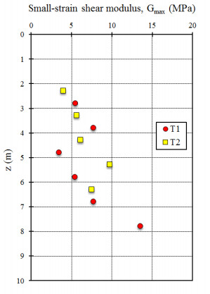
    [16] Mäenpää J (2016) Seismisen CPTU-mittauksen käyttö leikkausaallon nopeuden määrittämiseen. (In Finnish. Title in english: Determining Shear Wave Velocity by Seismic CPTU). M. Sc. Thesis, Tampere University of Technology, Finland.
    [17] SFS (2006) Finnish Standards: Geotechnical Investigation and Testing. Sampling Methods and Groundwater Measurements. Part 1. Technical Principles for Execution, SFS-EN ISO 22475-1:2006E, 120.
    [18] Mataic I (2016) On structure and rate dependence of Perniö clay. Doctoral dissertation, Ph. D. thesis, Department of Civil and Environmental Engineering, Aalto University, Helsinki, Finland.
    [19] Andresen A, Kolstad P (1980) The NGI 54-mm samplers for undisturbed sampling of clays and representative sampling of coarser material. NGI Publication No. 21, Norwegian Geotechnical Institute, Oslo, 1–31.
    [20] Larsson R (2011) Metodbeskrivning för SGI:s 200 mm diameter "blockprovtagare"-Ostörd Provtagning i finkornig jord (In Swedish), Swedish Geotechnical Institute (SGI). Göta River Commission, GÄU. Subreport 33. Linköping.
    [21] Lunne T, Berre T, Strandvik S (1997) Sample disturbance effects in soft low plastic Norwegian clay. In Proceedings of the Conference on Recent Developments in Soil and Pavement Mechanics, Rio de Janeiro, 81–102.
    [22] ISO (2004) ISO/TS 17892-12:2004 Geotechnical investigation and testing-Laboratory testing of soil-Part 12: Determination of Atterberg limits.
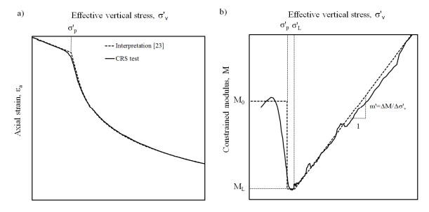
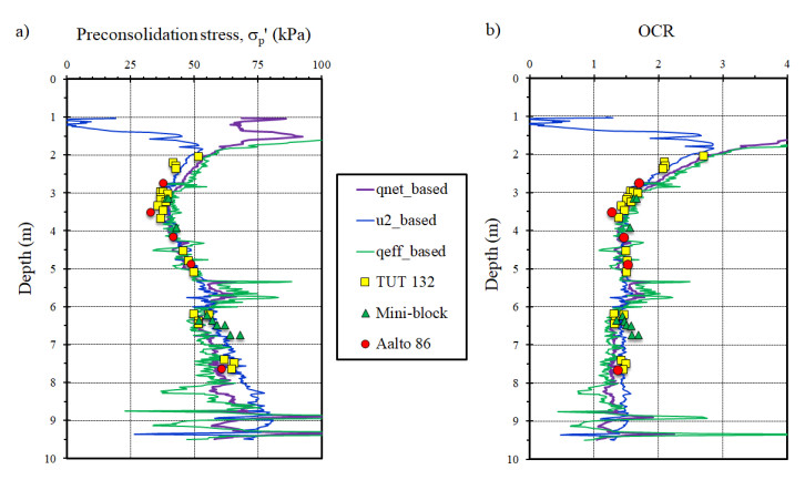
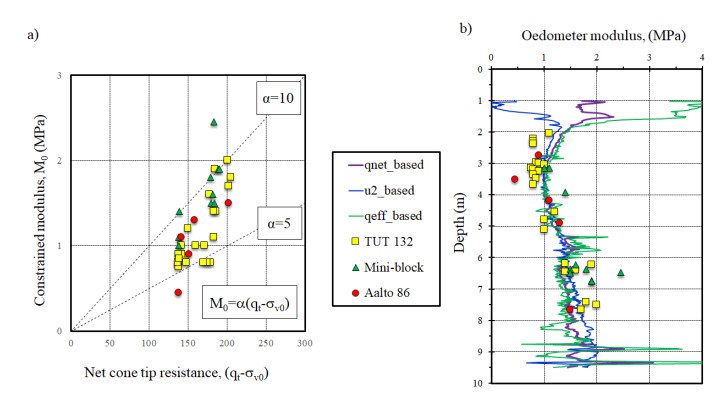
    [23] Kolisoja P, Sahi K, Hartikainen J (1989) An automatic triaxial-oedometer device. In Proceedings of the 12th International Conference on Soil Mechanics and Foundaiton Engineering, Rio De Janeiro, 61–64.
    [24] Sällfors G (1975) Preconsolidation pressure of soft, high-plastic clays. Doctoral dissertation, Chalmers University of Technology, Göteborg, Sweden.
    [25] Kulhawy FH, Mayne PW (1990) Manual on estimating soil properties for foundation design (No. EPRI-EL-6800). Electric Power Research Inst., Palo Alto, CA (USA); Cornell Univ., Ithaca, NY (USA).
    [26] Selänpää J (2019) A correlation to assess undrained shear strength by piezocone test for Finnish clay (CPTu). Doctoral dissertation, Ph. D. thesis, Tampere University, Tampere. Under review.
    [27] Selänpää J, Di Buò B, Haikola M, et al. (2018) Evaluation of existing CPTu-based correlations for the undrained shear strength of soft Finnish clays. In Cone Penetration Testing IV: Proceedings of the 4th International Symposium on Cone Penetration Testing (CPT 2018), Delft, CRC Press, 185–191.
    [28] Karlsrud K, Lunne T, Kort DA, et al. (2005) CPTU correlations for clays. In Proceedings of the international conference on soil mechanics and geotechnical engineering (Osaka). AA Balkema Publishers 16: 693.
    [29] Paniagua P, D'Ignazio M, L'Heureux JS, et al. (2019) CPTU correlations for Norwegian clays: an update. AIMS Geosci 5: 82–103. doi: 10.3934/geosci.2019.2.82
    [30] Karlsrud K, Hernandez-Martinez FG (2013) Strength and deformation properties of Norwegian clays from laboratory tests on high-quality block samples. Can Geotech J 50: 1273–1293. doi: 10.1139/cgj-2013-0298
    [31] D'Ignazio M, Phoon KK, Tan SA, et al. (2017) Reply to the discussion by Mesri and Wang on "Correlations for undrained shear strength of Finnish soft clays". Can Geotech J 54: 749–753. doi: 10.1139/cgj-2017-0114
    [32] Mayne PW (2005) Integrated ground behavior: in-situ and lab tests. Deformation Characteristics of Geomaterials, Taylor & Francis Group, London: 2.
    [33] Mayne PW (2007) NCHRP Synthesis 368 on Cone Penetration Testing. Transportation Research Board, Washington DC, 118.
    [34] Sanglerat G (1972)   The Penetrometer and Soil Exploration Interpretation of Penetration Diagrams-theory and Practice: Developments in Geotechnical Engineering 1. Elsevier.
    [35] Di Buò B, Selänpää J, Lansivaara,T, et al. (2018) Evaluation of existing CPTu-based correlations for the deformation properties of Finnish soft clays. In Cone Penetration Testing IV: Proceedings of the 4th International Symposium on Cone Penetration Testing (CPT 2018), Delft 185–191.
    [36] Mayne PW, Rix GJ (1995) Correlations between shear wave velocity and cone tip resistance in natural clays. Soils Found 35: 107–110. doi: 10.3208/sandf1972.35.2_107
    [37] Robertson PK (2009) Interpretation of cone penetration tests-a unified approach. Can Geotech J 46: 1337–1355. doi: 10.1139/T09-065
    [38] Mayne PW (2014) Interpretation of geotechnical parameters from seismic piezocone tests. In Proceedings of 3rd International Symposium on Cone Penetration Testing, CPT14, Las Vegas, Nevada, Gregg Drilling & Testing.
    [39] L'Heureux JS, Long M (2017) Relationship between shear-wave velocity and geotechnical parameters for Norwegian clays. J Geotech Geoenviron Eng 143: 04017013. doi: 10.1061/(ASCE)GT.1943-5606.0001645
    [40] Andersen KH, Schjetne K (2013) Database of friction angles of sand and consolidation characteristics of sand, silt, and clay. J Geotech Geoenviron Eng 139: 1140–1155. doi: 10.1061/(ASCE)GT.1943-5606.0000839
    [41] Länsivaara (2012) Some aspects on creep and primary deformation properties of soft sensitive Scandinavian clays. In Proceedings of the 16th Nordic Geotechnical Meeting, NGM, Copenhagen, Denmark, 9–12.
    [42] Janbu N (1963) Soil compressibility as determined by oedometer and triaxial tests. In Proceeding of the European Conference on Soil Mechanics and Foundation Engineering 1: 19–25.
  • This article has been cited by:

    1. Kamarul Amin Abdullah, Sara Marziali, Muzna Nanaa, Lorena Escudero Sánchez, Nicholas R. Payne, Fiona J. Gilbert, Deep learning-based breast cancer diagnosis in breast MRI: systematic review and meta-analysis, 2025, 1432-1084, 10.1007/s00330-025-11406-6
  • Reader Comments
  • © 2019 the Author(s), licensee AIMS Press. This is an open access article distributed under the terms of the Creative Commons Attribution License (http://creativecommons.org/licenses/by/4.0)
通讯作者: 陈斌, bchen63@163.com
  • 1. 

    沈阳化工大学材料科学与工程学院 沈阳 110142

  1. 本站搜索
  2. 百度学术搜索
  3. 万方数据库搜索
  4. CNKI搜索

Metrics

Article views(5769) PDF downloads(865) Cited by(8)

Figures and Tables

Figures(20)  /  Tables(4)

/

DownLoad:  Full-Size Img  PowerPoint
Return
Return

Catalog