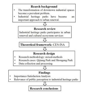
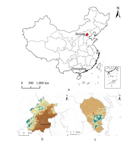
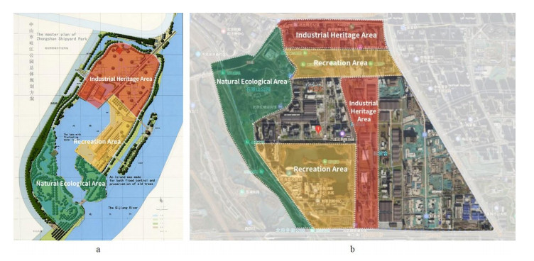
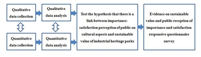
The transformation of downtown industrial spaces is prevalent in cities in China and the global South. Because of economic development and social transformation, former factories no longer carry out production activities and are abandoned. Industrial heritage parks, as integrated urban parks with new cultural and ecological paradigms, provide unique cultural ecosystem services (CES) that contribute to the sustainable development of urban renewal. Assessing their CES to identify public satisfaction is essential for urban green space planning and management and for enhancing human well-being. Thus, we tried to investigate public perceptions of CES in industrial heritage parks and explored the relationship between public satisfaction with CES and high-quality industrial heritage parks. Using importance-satisfaction analysis (ISA) to assess CES based on public perceptions, the cultural ecosystem services importance satisfaction analysis (CES-ISA) framework was established. Two successful examples of industrial heritage renewal in China, Qijiang Park, and Shougang Park were selected as case studies. The results indicated that: ⅰ) There is a positive correlation between public importance-satisfaction feedback at the cultural level and high quality industrial heritage parks; ⅱ) the recreational, aesthetic and cultural heritage, and spiritual services provided by industrial heritage parks were the types of CES most valued by the public; ⅲ) improving the sense of place service is key to enhancing public satisfaction and promoting the sustainability of industrial heritage parks; ${\rm{iiii}}$) the CES-ISA framework can identify differences between public perceptions of importance and satisfaction with CES. It is beneficial to obtain management priorities for cultural services in industrial heritage parks.
Citation: Sunny Han Han, Yujing Li, Peiheng Yu. What makes a successful industrial heritage park?—China's experience based on the ecosystem cultural services perspective[J]. Urban Resilience and Sustainability, 2024, 2(2): 93-109. doi: 10.3934/urs.2024006
The transformation of downtown industrial spaces is prevalent in cities in China and the global South. Because of economic development and social transformation, former factories no longer carry out production activities and are abandoned. Industrial heritage parks, as integrated urban parks with new cultural and ecological paradigms, provide unique cultural ecosystem services (CES) that contribute to the sustainable development of urban renewal. Assessing their CES to identify public satisfaction is essential for urban green space planning and management and for enhancing human well-being. Thus, we tried to investigate public perceptions of CES in industrial heritage parks and explored the relationship between public satisfaction with CES and high-quality industrial heritage parks. Using importance-satisfaction analysis (ISA) to assess CES based on public perceptions, the cultural ecosystem services importance satisfaction analysis (CES-ISA) framework was established. Two successful examples of industrial heritage renewal in China, Qijiang Park, and Shougang Park were selected as case studies. The results indicated that: ⅰ) There is a positive correlation between public importance-satisfaction feedback at the cultural level and high quality industrial heritage parks; ⅱ) the recreational, aesthetic and cultural heritage, and spiritual services provided by industrial heritage parks were the types of CES most valued by the public; ⅲ) improving the sense of place service is key to enhancing public satisfaction and promoting the sustainability of industrial heritage parks; ${\rm{iiii}}$) the CES-ISA framework can identify differences between public perceptions of importance and satisfaction with CES. It is beneficial to obtain management priorities for cultural services in industrial heritage parks.

| [1] | Zhu DJ (2018) Preface-Exploring the theoretical basis, indicator system and regional practice of global sustainable development goals. Bull Chin Acad Sci 33: 9. Available from: http://www.bulletin.cas.cn/thesisDetails?columnId=35527627&Fpath=home&index=0&lang=zh. |
| [2] | United Nations (2020) The Sustainable Development Goals Report 2020. Available from: https://sdgs.un.org/publications/sustainable-development-goals-report-2020-24686. |
| [3] | Han H (2023) The China Solution: 100 Stories of Industrial Heritage Conservation and Renewal. Wuhan: Huazhong University of Science and Technology Press. |
| [4] |
Zhang J, Cenci J, Becue V, et al. (2022) Analysis of spatial structure and influencing factors of the distribution of national industrial heritage sites in China based on mathematical calculations. Environ Sci Pollut Res 29: 27124–27139. https://doi.org/10.1007/s11356-021-17866-9 doi: 10.1007/s11356-021-17866-9

|
| [5] |
Zhang J, Cenci J, Becue V, et al. (2022) Stewardship of industrial heritage protection in typical Western European and Chinese regions: Values and dilemmas. Land 11: 772. https://doi.org/10.3390/land11060772 doi: 10.3390/land11060772
|
| [6] | Roberts P, Sykes H (2000) Urban Regeneration: A Hand-book. London: SAGE Publications. |
| [7] |
Pozen MW, Goshin AR, Bellin LE (1968) Evaluation of housing standards of families within four years of relocation by urban renewal. Am J Public Health 58: 1256–1264. https://doi.org/10.2105/AJPH.58.7.1256 doi: 10.2105/AJPH.58.7.1256
|
| [8] |
Knittel RE (1963) The effect of urban renewal on community development. Am J Public Health 53: 67–70. https://doi.org/10.2105/AJPH.53.1.67 doi: 10.2105/AJPH.53.1.67
|
| [9] |
Lee BA, Spain D, Umberson DJ (1985) Neighborhood revitalization and racial change: The case of Washington, DC. Demography 22: 581–602. https://doi.org/10.2307/2061589 doi: 10.2307/2061589
|
| [10] |
Silvers AH (1969) Urban renewal and black power. Am Behav Sci 12: 43–46. https://doi.org/10.1177/000276426901200409 doi: 10.1177/000276426901200409
|
| [11] |
Hackworth J, Smith N (2001) The changing state of gentrification. J Econ Hum Geogr 92: 464–477. https://doi.org/10.1111/1467-9663.00172 doi: 10.1111/1467-9663.00172
|
| [12] |
Foley P, Martin S (2000) A new deal for the community? Public participation in regeneration and local service delivery. Policy Polit 28: 479–492. https://doi.org/10.1332/0305573002501090 doi: 10.1332/0305573002501090
|
| [13] |
Lowndes V, Skelcher C (1998) The dynamics of multi‐organizational partnerships: an analysis of changing modes of governance. Public Adm 76: 313–333. https://doi.org/10.1111/1467-9299.00103 doi: 10.1111/1467-9299.00103
|
| [14] |
Zheng HW, Shen GQ, Wang H (2014) A review of recent studies on sustainable urban renewal. Habitat Int 41: 272–279. https://doi.org/10.1016/j.habitatint.2013.08.006 doi: 10.1016/j.habitatint.2013.08.006
|
| [15] | Cossons N (2012) Why preserve the industrial heritage, In: Industrial Heritage Re-Tooled: The TICCIH Guide to Industrial Heritage Conservation, London: Routledg, 6–16. |
| [16] |
Gallagher F, Goodey NM, Hagmann D, et al. (2018) Urban re-greening: a case study in multi-trophic biodiversity and ecosystem functioning in a post-industrial landscape. Diversity 10: 119–133. https://doi.org/10.3390/d10040119 doi: 10.3390/d10040119
|
| [17] | Prentice RC, Witt SF, Hamer C (1993) The experience of industrial heritage: The case of Black Gold. Built Environ 19: 137–146. |
| [18] | Alfrey J, Putnam T (2003) The Industrial Heritage: Managing Resources and Uses. London: Routledge. https://doi.org/10.4324/9780203392911 |
| [19] |
Zhang J, Cenci J, Becue V, et al. (2021) The overview of the conservation and renewal of the industrial Belgian heritage as a vector for cultural regeneration. Information 12: 27. https://doi.org/10.3390/info12010027 doi: 10.3390/info12010027
|
| [20] |
Zhang J, Cenci J, Becue V (2021) A preliminary study on industrial landscape planning and spatial layout in Belgium. Heritage 4: 1375–1387. https://doi.org/10.3390/heritage4030075 doi: 10.3390/heritage4030075
|
| [21] | Assessment ME (2003) Ecosystems and Human Well-being: A Framework for Assessment. Millennium Ecosystem Assessment. |
| [22] |
Yu P, Zhang S, Yung EHK, et al. (2023) On the urban compactness to ecosystem services in a rapidly urbanising metropolitan area: Highlighting scale effects and spatial non-stationary. Environ Impact Assess Rev 98: 106975. https://doi.org/10.1016/j.eiar.2022.106975 doi: 10.1016/j.eiar.2022.106975
|
| [23] |
Gómez-Baggethun E, Barton DN (2013) Classifying and valuing ecosystem services for urban planning. Ecol Econ 86: 235–245. https://doi.org/10.1016/j.ecolecon.2012.08.019 doi: 10.1016/j.ecolecon.2012.08.019
|
| [24] |
Kaba S, Kojima M, Matsuda H, et al. (2006) Küttner's tumor of the submandibular glands: Report of five cases with fine-needle aspiration cytology. Diagn Cytopathol 34: 631–635. https://doi.org/10.1002/dc.20505 doi: 10.1002/dc.20505
|
| [25] |
Helliwell DR (1969) Valuation of wildlife resources. Reg Stud 3: 41–47. https://doi.org/10.1080/09595236900185051 doi: 10.1080/09595236900185051
|
| [26] |
Costanza R, d'Arge R, De Groot R, et al. (1997) The value of the world's ecosystem services and natural capital. Nature 387: 253–260. https://doi.org/10.1038/387253a0 doi: 10.1038/387253a0
|
| [27] |
Zhao Q, Li J, Liu J, et al. (2018) Assessment and analysis of social values of cultural ecosystem services based on the SolVES model in the Guanzhong-Tianshui Economic Region. Acta Ecol Sin 38: 3673–3681. https://doi.org/10.5846/stxb201704240738 doi: 10.5846/stxb201704240738
|
| [28] |
Huo SG, Huang L, Yan L (2018) Valuation of cultural ecosystem services based on SolVES: a case study of the South Ecological Park in Wuyi County, Zhejiang Province. Acta Ecol Sin 38: 3682–3691. https://doi.org/10.5846/stxb201704110624 doi: 10.5846/stxb201704110624
|
| [29] | Church A, Fish R, Haines-Young R, et al. (2014) UK national ecosystem assessment follow-on work package report 5: Cultural ecosystem services and indicators. Available from: http://uknea.unep-wcmc.org/Resources/tabid/82/Default.aspx. |
| [30] |
Daniel TC, Muhar A, Arnberger A, et al. (2012) Contributions of cultural services to the ecosystem services agenda. Proc Natl Acad Sci 109: 8812–8819. https://doi.org/10.1073/pnas.1114773109 doi: 10.1073/pnas.1114773109
|
| [31] |
Hernández-Morcillo M, Plieninger T, Bieling C (2013) An empirical review of cultural ecosystem service indicators. Ecol Indic 29: 434–444. https://doi.org/10.1016/j.ecolind.2013.01.013 doi: 10.1016/j.ecolind.2013.01.013
|
| [32] |
Tonge J, Moore SA (2007) Importance-satisfaction analysis for marine park hinterlands: A Western Australian case study. Tour Manag 28: 768–776. https://doi.org/10.1016/j.tourman.2006.05.007 doi: 10.1016/j.tourman.2006.05.007
|
| [33] |
Taplin RH (2012) Competitive importance-performance analysis of an Australian wildlife park. Tour Manag 33: 29–37. https://doi.org/10.1016/j.tourman.2011.01.020 doi: 10.1016/j.tourman.2011.01.020
|
| [34] |
Galaz-Mandakovic D, Rivera F (2023) The industrial heritage of two sacrifice zones and the geopolitics of memory in Northern Chile. The cases of Gatico and Ollagüe. Int J Heritage Stud 29: 243–259. https://doi.org/10.1080/13527258.2023.2181379 doi: 10.1080/13527258.2023.2181379
|
| [35] |
Leung MWH, Soyez D (2009) Industrial heritage: Valorising the spatial–temporal dynamics of another Hong Kong story. Int J Heritage Stud 15: 57–75. https://doi.org/10.1080/13527250902746096 doi: 10.1080/13527250902746096
|
| [36] |
Qian Z (2023) Heritage conservation as a territorialised urban strategy: Conservative reuse of socialist industrial heritage in China. Int J Heritage Stud 29: 63–80. https://doi.org/10.1080/13527258.2023.2169954 doi: 10.1080/13527258.2023.2169954
|
| [37] |
El-Husseiny MA, Kesseiba K (2012) Challenges of social sustainability in neo-liberal Cairo: Re-questioning the role of public space. Procedia Soc Behav Sci 68: 790–803. https://doi.org/10.1016/j.sbspro.2012.12.267 doi: 10.1016/j.sbspro.2012.12.267
|
| [38] |
Boland P, Durrant A, McHenry J, et al. (2022) A 'planning revolution' or an 'attack on planning' in England: Digitization, digitalization, and democratization. Int Plan Stud 27: 155–172. https://doi.org/10.1080/13563475.2021.1979942 doi: 10.1080/13563475.2021.1979942
|
| [39] |
Fuseini I (2021) Decentralisation, entrepreneurialism and democratization processes in urban governance in Tamale, Ghana. Area Dev Policy 6: 223–242. https://doi.org/10.1080/23792949.2020.1750303 doi: 10.1080/23792949.2020.1750303
|
| [40] |
Chigbu UE, Ntihinyurwa PD, de Vries WT, et al. (2019) Why tenure responsive land-use planning matters: Insights for land use consolidation for food security in Rwanda. Int J Environ Res Public Health 16: 1354. https://doi.org/10.3390/ijerph16081354 doi: 10.3390/ijerph16081354
|
| [41] |
Ntihinyurwa PD, de Vries WT, Chigbu UE, et al. (2019) The positive impacts of farm land fragmentation in Rwanda. Land Use Policy 81: 565–581. https://doi.org/10.1016/j.landusepol.2018.11.005 doi: 10.1016/j.landusepol.2018.11.005
|
| [42] |
Yu P, Fennell S, Chen Y, et al. (2022) Positive impacts of farmland fragmentation on agricultural production efficiency in Qilu Lake watershed: Implications for appropriate scale management. Land Use Policy 117: 106108. https://doi.org/10.1016/j.landusepol.2022.106108 doi: 10.1016/j.landusepol.2022.106108
|
| [43] |
Li CH, Sun YH, Jia YH, et al. (2010) Analytic hierarchy process based on variable weights. Syst Eng Theory Pract 30: 723–731. https://doi.org/10.12011/1000-6788(2010)4-723 doi: 10.12011/1000-6788(2010)4-723
|
| [44] |
Li K, Shen W, Huang ZS (2019) Performance evaluation of culture ecosystem services of urban green space: A case study on Qianlingshan Park of Guiyang City. Urban Probl 2019: 44–50. https://doi.org/10.13239/j.bjsshkxy.cswt.190306 doi: 10.13239/j.bjsshkxy.cswt.190306
|
| [45] | Steele F (1981) The Sense of Place. Boston: CBI Publishing. |
| [46] |
Khew JYT, Yokohari M, Tanaka T (2014) Public perceptions of nature and landscape preference in Singapore. Hum Ecol 42: 979–988. https://doi.org/10.1007/s10745-014-9709-x doi: 10.1007/s10745-014-9709-x
|
| [47] |
Gobster PH, Nassauer JI, Daniel TC, et al. (2007) The shared landscape: What does aesthetics have to do with ecology? Landsc Ecol 22: 959–972. https://doi.org/10.1007/s10980-007-9110-x doi: 10.1007/s10980-007-9110-x
|
| [48] | Tang Y, Wang YS, Fu YY, et al. (2019) Memorial Landscapes of Earthquake: Landscape Perception and Sense of Place. Chengdu: Sichuan University Press. |
Figures(4) / Tables(5)
Sunny Han Han, Yujing Li, Peiheng Yu. What makes a successful industrial heritage park?—China's experience based on the ecosystem cultural services perspective[J]. Urban Resilience and Sustainability, 2024, 2(2): 93-109. doi: 10.3934/urs.2024006


 DownLoad: