Emerging pollutants in the environment due to economic development have become a global challenge for environmental and human health management. Potentially toxic elements (PTEs), a major group of pollutants, have been detected in soil, air, water and food crops. Humans are exposed to PTEs through soil ingestion, consumption of water, uptake of food crop products originating from polluted fields, breathing of dust and fumes, and direct contact of the skin with contaminated soil and water. The dose absorbed by humans, the exposure route and the duration (i.e., acute or chronic) determine the toxicity of PTEs. Poisoning by PTEs can lead to excessive damage to health as a consequence of oxidative stress produced by the formation of free radicals and, as a consequence, to various disorders. The toxicity of certain organs includes neurotoxicity, nephrotoxicity, hepatotoxicity, skin toxicity, and cardiovascular toxicity. In the treatment of PTE toxicity, synthetic chelating agents and symptomatic supportive procedures have been conventionally used. In addition, there are new insights concerning natural products which may be a powerful option to treat several adverse consequences. Health policy implications need to include monitoring air, water, soil, food products, and individuals at risk, as well as environmental manipulation of soil, water, and sewage. The overall goal of this review is to present an integrated view of human exposure, risk assessment, clinical effects, as well as therapy, including new treatment options, related to highly toxic PTEs.
Citation: Rolf Nieder, Dinesh K. Benbi. Integrated review of the nexus between toxic elements in the environment and human health[J]. AIMS Public Health, 2022, 9(4): 758-789. doi: 10.3934/publichealth.2022052
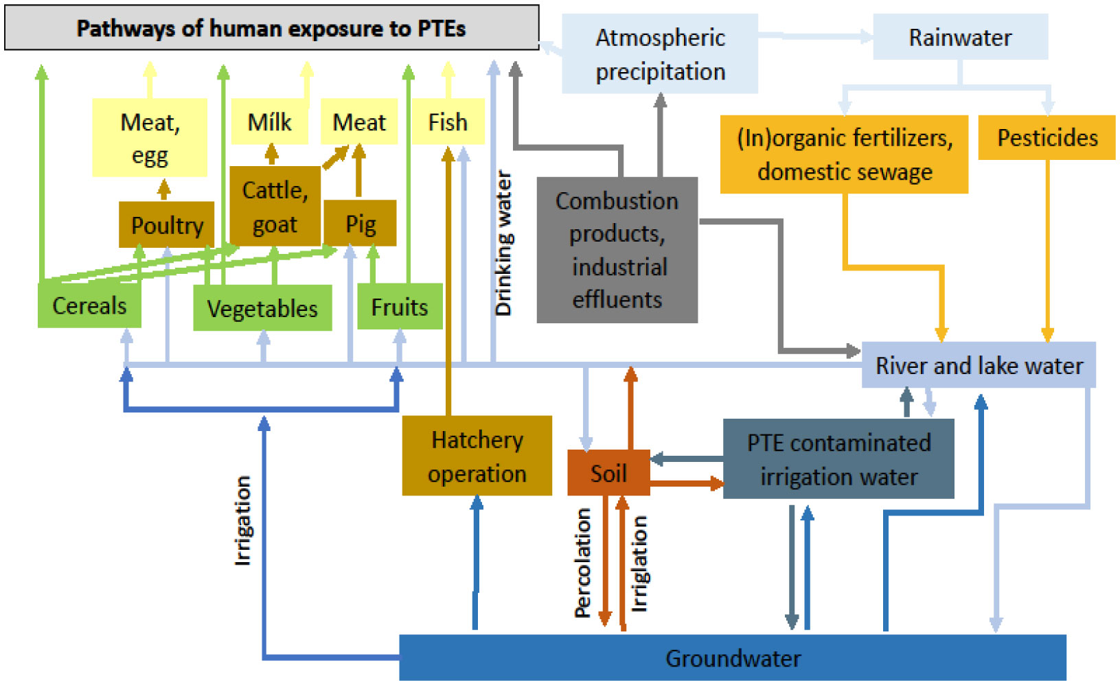
Emerging pollutants in the environment due to economic development have become a global challenge for environmental and human health management. Potentially toxic elements (PTEs), a major group of pollutants, have been detected in soil, air, water and food crops. Humans are exposed to PTEs through soil ingestion, consumption of water, uptake of food crop products originating from polluted fields, breathing of dust and fumes, and direct contact of the skin with contaminated soil and water. The dose absorbed by humans, the exposure route and the duration (i.e., acute or chronic) determine the toxicity of PTEs. Poisoning by PTEs can lead to excessive damage to health as a consequence of oxidative stress produced by the formation of free radicals and, as a consequence, to various disorders. The toxicity of certain organs includes neurotoxicity, nephrotoxicity, hepatotoxicity, skin toxicity, and cardiovascular toxicity. In the treatment of PTE toxicity, synthetic chelating agents and symptomatic supportive procedures have been conventionally used. In addition, there are new insights concerning natural products which may be a powerful option to treat several adverse consequences. Health policy implications need to include monitoring air, water, soil, food products, and individuals at risk, as well as environmental manipulation of soil, water, and sewage. The overall goal of this review is to present an integrated view of human exposure, risk assessment, clinical effects, as well as therapy, including new treatment options, related to highly toxic PTEs.

| [1] | Coccia M, Bellitto M (2018) Human progress and its socioeconomic effects in society. JEST 5: 160-178. |
| [2] | Coccia M (2019) Comparative Institutional Changes. Global Encyclopedia of Public Administration, Public Policy, and Governance . Springer Nature. https://doi.org/10.1007/978-3-319-31816-5_1277-1 |
| [3] | Coccia M (2018) An introduction to the theories of national and regional economic development. TER 5: 350-358. https://doi.org/10.2139/ssrn.3857165 |
| [4] | Coccia M (2021) Effects of human progress driven by technological change on physical and mental health. Studi Sociol 2: 113-132. |
| [5] |
Coccia M (2015) The Nexus between technological performances of countries and incidence of cancers in society. Technol Soc 42: 61-70. https://doi.org/10.1016/j.techsoc.2015.02.003 
|
| [6] |
Irigaray P, Newby JA, Clapp R, et al. (2007) Lifestyle-related factors and environmental agents causing cancer: an overview. Biomed Pharmacother 61: 640-658. https://doi.org/10.1016/j.biopha.2007.10.006
|
| [7] |
Coccia M (2013) The effect of country wealth on incidence of breast cancer. Breast Cancer Res Treat 141: 225-229. https://doi.org/10.1007/s10549-013-2683-y
|
| [8] |
Coccia M (2020) Factors determining the diffusion of COVID-19 and suggested strategy to prevent future accelerated viral infectivity similar to COVID. Sci Total Environ 729: 138474. https://doi.org/10.1016/j.scitotenv.2020.138474
|
| [9] |
Núñez-Delgado A, Bontempi E, Coccia M, et al. (2021) SARS-CoV-2 and other pathogenic microorganisms in the environment. Environ Res 201: 111606. https://doi.org/10.1016/j.envres.2021.111606
|
| [10] | Chang LW, Magos L, Suzuki T (1996) Toxicology of Metals. Boca Raton, FL, USA: CRC Press. |
| [11] |
Prabhakaran KP, Cottenie A (1971) Parent material - soil relationship in trace elements - a quantitative estimation. Geoderma 5: 81-97. https://doi.org/10.1016/0016-7061(71)90014-0
|
| [12] |
Khan S, Cao Q, Zheng YM, et al. (2008) Health risks of heavy metals in contaminated soils and food crops irrigated with wastewater in Beijing, China. Environ Poll 152: 686-692. https://doi.org/10.1016/j.envpol.2007.06.056
|
| [13] | Wuana RA, Okieimen FE (2011) Heavy metals in contaminated soils: a review of sources, chemistry, risks and best available strategies for remediation. International Scholarly Research Network ISRN Ecology . https://doi.org/10.5402/2011/402647 |
| [14] |
Li G, Sun GX, Ren Y, et al. (2018) Urban soil and human health: a review. Eur J Soil Sci 69: 196-215. https://doi.org/10.1111/ejss.12518
|
| [15] |
Nieder R, Benbi DK, Reichl FX (2018) Soil Components and Human Health. Dordrecht: Springer. https://doi.org/10.1007/978-94-024-1222-2
|
| [16] |
Rinklebe J, Antoniadis V, Shaheen SM, et al. (2019) Health risk assessmant of potentially oxic elements in soils along the Elbe River, Germany. Environ Int 126: 76-88. https://doi.org/10.1016/j.envint.2019.02.011
|
| [17] | Pohl WL (2020) Economic Geology. Principles and Practice. Stuttgart: Schweizerbart Science Publishers. |
| [18] | GWRTACRemediation of metals-contaminated soils and groundwater, Tech Rep TE-97-01, GWRTAC, Pittsburgh, Pa, USA, 1997, GWRTAC-E Series (1997). |
| [19] |
Aslanidis PSC, Golia EE (2022) Urban Sustainability at Risk Due to Soil Pollution by Heavy Metals—Case Study: Volos, Greece. Land 11: 1016. https://doi.org/10.3390/land11071016
|
| [20] |
Golia EE, Papadimou SG, Cavalaris C, et al. (2021) Level of Contamination Assessment of Potentially Toxic Elements in the Urban Soils of Volos City (Central Greece). Sustainability 13: 2029. https://doi.org/10.3390/su13042029
|
| [21] |
Serrani D, Ajmone-Marsan F, Corti G, et al. (2022) Heavy metal load and effects on biochemical properties in urban soils of a medium-sized city, Ancona, Italy. Environ Geochem Health 44: 3425-3449. https://doi.org/10.1007/s10653-021-01105-8
|
| [22] | Ndoli A, Naramabuye F, Diogo RV, et al. (2013) Greenhouse experiments on soybean (Glycine max) growth on Technosol substrates from tantalum mining in Rwanda. Int J Agric Sci 2: 144-152. |
| [23] |
Nieder R, Weber TKD, Paulmann I, et al. (2014) The geochemical signature of rare-metal pegmatites in the Central Africa Region: Soils, plants, water and stream sediments in the Gatumba tin-tantalum mining district, Rwanda. J Geochem Explor 144: 539-551. https://doi.org/10.1016/j.gexplo.2014.01.025
|
| [24] | Reetsch A, Naramabuye F, Pohl W, et al. (2008) Properties and quality of soils in the open-cast mining district of Gatumba, Rwanda. Etudes Rwandaises 16: 51-79. |
| [25] |
Rossiter, DG (2007) Classification of Urban and Industrial Soils in the World Reference Base for Soil Resources. J Soils Sediments 7: 96-100. https://doi.org/10.1065/jss2007.02.208
|
| [26] |
Guo G, Li K, Lei M (2022) Accumulation, environmental risk characteristics and associated driving mechanisms of potential toxicity elements in roadside soils across China. Sci Total Environ 835: 155342. https://doi.org/10.1016/j.scitotenv.2022.155342
|
| [27] |
Antoniadis V, Levizou E, Shaheen SM, et al. (2017) Trace elements in the soil-plant interface: phytoavailability, translocation, and phytoremediation – a review. Earth Sci Rev 171: 621-645. https://doi.org/10.1016/j.earscirev.2017.06.005
|
| [28] | US EPA (Environmental Protection Agency)Reducing mercury pollution from gold mining (2011). Available from: http://www.epa.gov/oia/toxics/asgm.html. |
| [29] |
Pelfrêne A, Waterlot C, Mazzuca M, et al. (2012) Bioaccessibility of trace elements as affected by soil parameters in smelter-contaminated agricultural soils: A statistical modeling approach. Environ Pollut 160: 130-138. https://doi.org/10.1016/j.envpol.2011.09.008
|
| [30] |
Bolan N, Kunhikrishnan A, Thangarajan R, et al. (2014) Remediation of heavy metal(loid) contaminated soils – to mobilize or not to mobilize?. J Hazar Mater 266: 141-166. https://doi.org/10.1016/j.jhazmat.2013.12.018
|
| [31] | Tong S, von Schirnding YE, Prapamontol T (2000) Environmental lead exposure: a public health problem of global dimensions. Bulletin of the World Health Organization 78: 1068-1077. |
| [32] |
Järup L, Hellström L, Alfvén T, et al. (2000) Low level exposure to cadmium and early kidney damage: the OSCAR study. Occup Environ Med 57: 668-672. https://doi.org/10.1136/oem.57.10.668
|
| [33] |
Thomas LDK, Hodgson S, Nieuwenhuijsen M, et al. (2009) Early kidney damage in a population exposed to cadmium and other heavy metals. Environ Health Perspect 117: 181-184. https://doi.org/10.1289/ehp.11641
|
| [34] |
Putila JJ, Guo NL (2011) Association of arsenic exposure with lung cancer incidence rates in the United States. PLOS ONE 6: e25886. https://doi.org/10.1371/journal.pone.0025886
|
| [35] | WHO (World Health Organization)News Release, Geneva (2016). Available from: http://www.who.int/news-room/detail/15-03-2016-an-estimated-12-6-million-deaths-each-year-are-attributable-to-unhealthy-environments. |
| [36] |
Liu P, Zhang Y, Feng N, et al. (2020) Potentially toxic element (PTE) levels in maize, soil, and irrigation water and health risks through maize consumption in northern Ningxia, China. BMC Public Health 20: 1729. https://doi.org/10.1186/s12889-020-09845-5
|
| [37] | Mazumder D (2008) Chronic arsenic toxicity and human health. Indian J Med Res 128: 436-47. |
| [38] | Bires J, Dianovsky J, Bartko P, et al. (1995) Effects on enzymes and the genetic apparatus of sheep after administration of samples from industrial emissions. Biol Met 8: 53-58. https://doi.org/10.1007/BF00156158 |
| [39] |
Bolan S, Kunhikrishnan A, Seshadri B, et al. (2017) Sources, distribution, bioavailability, toxicity, and risk assessment of heavy metal(loid)s in complementary medicines. Environ Int 108: 103-118. https://doi.org/10.1016/j.envint.2017.08.005
|
| [40] | Rajkumar V, Gupta V (2022) Heavy Metal Toxicity. Treasure Island (FL): StatPearls Publishing 2022. Available from: https://www.ncbi.nlm.nih.gov/books/NBK560920/. |
| [41] | (2000) ATSDR (Agency for Toxic Substances and Disease Registry)Toxicological Profile for Arsenic. Georgia: Center for Disease Control, Atlanta. |
| [42] | Tchounwou PB, Yedjou CG, Patlolla AK, et al. (2012) Heavy metal toxicity and the environment. Exp Suppl 101: 133-164. https://doi.org/10.1007/978-3-7643-8340-4_6 |
| [43] | (2001) WHO (World Health Organization)Arsenic and Arsenic Compounds. Environmental Health Criteria 224 . Geneva: . Available from: http://www.inchem.org/documents/ehc/ehc/ehc224.htm |
| [44] |
Ravenscroft P, Brammer H, Richards K (2009) Arsenic Pollution: A Global Synthesis. West Sussex, UK: John Wiley and Sons. https://doi.org/10.1002/9781444308785
|
| [45] |
Shakoor MB, Niazi NK, Bibi I, et al. (2019) Exploring the arsenic removal potential of various biosorbents from water. Environ Int 123: 567-579. https://doi.org/10.1016/j.envint.2018.12.049
|
| [46] |
Shresther RR, Upadhyay NP, Pradhan R, et al. (2003) Groundwater arsenic contamination, its health impact and mitigation program in Nepal. J Environ Sci Health A38: 185-200. https://doi.org/10.1081/ESE-120016888
|
| [47] |
Berg M, Trans HC, Nguyeu TC, et al. (2001) Arsenic contamination of groundwater and drinking water in Vietnam: a human health threat. Environ Sci Technol 35: 2621-2626. https://doi.org/10.1021/es010027y
|
| [48] | Morton WE, Dunnette DA (1994) Health effects of environmental arsenic. Arsenic in the Environment Part II: Human Health and Ecosystem Effects . New York: John Wiley & Sons 17-34. |
| [49] |
Zhao KL, Liu XM, Xu JM, et al. (2010) Heavy metal contaminations in a soil–rice system: Identification of spatial dependence in relation to soil properties of paddy fields. J Hazard Mater 181: 778-787. https://doi.org/10.1016/j.jhazmat.2010.05.081
|
| [50] |
Williams PN, Islam MR, Adomako EE, et al. (2006) Increase in rice grain arsenic for regions of Bangladesh irrigating paddies with elevated arsenic in ground waters. Environ Sci Technol 40: 4903-4908. https://doi.org/10.1021/es060222i
|
| [51] |
Tchounwou PB, Centeno JA, Patlolla AK (2004) Arsenic toxicity, mutagenesis and carcinogenesis - a health risk assessment and management approach. Mol Cell Biochem 255: 47-55.
|
| [52] |
Concha G, Vogler G, Nermell B, et al. (1998) Low-level arsenic excretion inbreast milk of native Andean women exposed to high levels of arsenic in the drinking water. Int Arch Occup Environ Health 71: 42-46.
|
| [53] |
Dakeishi M, Murata K, Grandjean P (2006) Long-term consequences of arsenic poisoning during infancy due to contaminated milk powder. Environ Health 5: 31.
|
| [54] |
Järup L, Åkesson A (2009) Current status of cadmium as an environmental healthproblem. Toxicol Appl Pharm 238: 201-208.
|
| [55] |
Inaba T, Kobayashi E, Suwazono Y, et al. (2005) Estimation of cumulative cadmium intake causing Itai-itai disease. Toxicol Lett 159: 192-201.
|
| [56] |
Skinner HCW (2007) The earth, source of health and hazards: An introduction to Medical Geology. Annu Rev Earth Planet Sci 35: 177-213.
|
| [57] |
Nakagawa H, Tabata M, Moikawa Y, et al. (1990) High mortality and shortened life-span in patients with itai-itai disease and subjects with suspected disease. Arch Environ Health 45: 283-287.
|
| [58] |
Horiguchi H, Oguma E, Sasaki S, et al. (2004) Comprehensive study of the effects of age, iron deficiency, diabetes mellitus and cadmium burden on dietary cadmium absorption in cadmium-exposed female Japanese farmers. Toxicol Appl Pharmacol 196: 114-123.
|
| [59] |
Diamond GL, Thayer WC, Choudhury H (2003) Pharmacokinetic/pharmacodynamics (PK/PD) modeling of risks of kidney toxicity from exposure to cadmium: estimates of dietary risks in the U.S. population. J Toxicol Environ Health 66: 2141-2164.
|
| [60] |
Dayan AD, Paine AJ (2001) Mechanisms of chromium toxicity, carcinogenicity and allergenicity: Review of the literature from 1985 to 2000. Hum Exp Toxicol 20: 439-451.
|
| [61] |
Coetzee JJ, Bansal N, Evans M N, et al. (2020) Chromium in environment, its toxic effect from chromite-mining and ferrochrome industries, and its possible bioremediation. Expos Health 12: 51-62. https://doi.org/10.1007/s12403-018-0284-z
|
| [62] | Holmes AL, Wise SS, Wise JP (2008) Carcinogenicity of hexavalent chromium. Indian J Med Res 128: 353-357. |
| [63] | IARC (International Agency for Research on Cancer).Chromium, Nickel and Welding. IARC Monographs on the Evaluation of Carcinogenic Risks to Humans (1990) 49: 249-256. |
| [64] | Zhang JD, Li XL (1987) Chromium pollution of soil and water in Jinzhou. Zhonghua Yu Fang Yi Xue Za Zhi 21: 262-264. |
| [65] |
Barregard L, Sallsten G, Conradi N (1999) Tissue levels of mercury determined in a deceased worker after occupational exposure. Int Arch Occup Environ Health 72: 169-173. https://doi.org/10.1007/s004200050356
|
| [66] |
Ralston NVC, Raymond LJ (2018) Mercury's neurotoxicity is characterized by its disruption of selenium biochemistry. Biochim Biophys Acta Gen Subj 1862: 2405-2416. https://doi.org/10.1016/j.bbagen.2018.05.009
|
| [67] |
Sall ML, Diaw AKD, Gningue-Sall D, et al. (2020) Toxic heavy metals: impact on the environment and human health, and treatment with conducting organic polymers, a review. Environ Sci Pollut Res 27: 29927-29942. https://doi.org/10.1007/s11356-020-09354-3
|
| [68] |
Ekino S, Susa M, Ninomiya T, et al. (2007) Minamata disease revisited: An update on the acute and chronic manifestations of methyl mercury poisoning. J Neurol Sci 262: 131-144. https://doi.org/10.1016/j.jns.2007.06.036
|
| [69] |
Eto K (2000) Minamata disease. Neuropathol 20: S14-S19. https://doi.org/10.1046/j.1440-1789.2000.00295.x
|
| [70] |
Babut M, Sekyi R (2003) Improving the environmental management of small-scale gold mining in Ghana: a case study of Dumasi. J Cleaner Prod 11: 215-221. https://doi.org/10.1016/S0959-6526(02)00042-2
|
| [71] |
Taylor H, Appleton JD, Lister R, et al. (2004) Environmental assessment of mercury contamination from the Rwamagasa artisanal gold mining centre, Geita District, Tanzania. Sci Total Environ 343: 111-133. https://doi.org/10.1016/j.scitotenv.2004.09.042
|
| [72] | WHO (World Health Organization)Lead poisoning and health (2018). Available from: https://www.who.int/news-room/fact-sheets/detail/lead-poisoning-and-health |
| [73] |
O'Connor D, Hou D, Ye J, et al. (2018) Lead-based paint remains a major public health concern: a critical review of global production, trade, use, exposure, health risk, and implications. Environ Int 121: 85-101. https://doi.org/10.1016/j.envint.2018.08.052
|
| [74] |
Järup L (2003) Hazards of heavy metal contamination. Brit Med Bull 68: 67-182. https://doi.org/10.1093/bmb/ldg032
|
| [75] |
Shifaw E (2018) Review of Heavy Metals Pollution in China in Agricultural and Urban Soils. J Health Pollut 8: 180607. https://doi.org/10.5696/2156-9614-8.18.180607
|
| [76] |
Wang W, Xu X, Zhou Z, et al. (2022) A joint method to assess pollution status and source-specific human health risks of potential toxic elements in soils. Environ Monit Assess 194: 685. https://doi.org/10.1007/s10661-022-10353-9
|
| [77] |
Lei M, Li K, Guo G, et al. (2022) Source-specific health risks apportionment of soil potential toxicity elements combining multiple receptor models with Monte Carlo simulation. Sci Total Environ 817: 152899. https://doi.org/10.1016/j.scitotenv.2021.152899
|
| [78] |
Xue S, Korna R, Fan J, et al. (2023) Spatial distribution, environmental risks, and sources of potentially toxic elements in soils from a typical abandoned antimony smelting site. J Environ Sci 127: 780-790. https://doi.org/10.1016/j.jes.2022.07.009
|
| [79] |
Mohammadpour A, Emadi Z, Keshtkar M, et al. (2022) Assessment of potentially toxic elements (PTEs) in fruits from Iranian market (Shiraz): A health risk assessment study. J Food Compost Anal 114: 104826. https://doi.org/10.1016/j.jfca.2022.104826
|
| [80] |
Vejvodová K, Ash C, Dajčl J, et al. (2022) Assessment of potential exposure to As, Cd, Pb and Zn in vegetable garden soils and vegetables in a mining region. Sci Rep 12: 13495. https://doi.org/10.1038/s41598-022-17461-z
|
| [81] |
Natasha N, Shahid M, Murtaza B, et al. (2022) Accumulation pattern and risk assessment of potentially toxic elements in selected wastewater-irrigated soils and plants in Vehari, Pakistan. Environ Res 214: 114033. https://doi.org/10.1016/j.envres.2022.114033
|
| [82] |
Ghane ET, Khanverdiluo S, Mehri F (2022) The concentration and health risk of potentially toxic elements (PTEs) in the breast milk of mothers: a systematic review and meta-analysis. J Trace Elem Med Biol 73: 126998. https://doi.org/10.1016/j.jtemb.2022.126998
|
| [83] |
DeForest DK, Brix KV, Adams WJ (2007) Assessing metal bioaccumulation in aquatic environments: the inverse relationship between bioaccumulation factors, trophic transfer factors and exposure concentration. Aquat Toxicol 84: 236-246. https://doi.org/10.1016/j.aquatox.2007.02.022
|
| [84] |
Wang S, Shi X (2001) Molecular mechanisms of metal toxicity and carcinogenesis. Mol Cell Biochem 222: 3-9. https://doi.org/10.1023/A:1017918013293
|
| [85] |
Ercal N, Gurer-Orhan H, Aykin-Burns N (2001) Toxic metals and oxidative stress Part I: mechanisms involved in metal-induced oxidative damage. Curr Top Med Chem 1: 529-539. https://doi.org/10.2174/1568026013394831
|
| [86] |
Wilk A, Kalisinska E, Kosik-Bogacka DI, et al. (2017) Cadmium, lead and mercury concentrations in pathologically altered human kidneys. Environ Geochem Health 39: 889-899. https://doi.org/10.1007/s10653-016-9860-y
|
| [87] |
Ebrahimpour M, Mosavisefat M, Mohabatti R (2010) Acute toxicity bioassay of mercuric chloride: an alien fish from a river. Toxicol Environ Chem 92: 169-173. https://doi.org/10.1080/02772240902794977
|
| [88] | Brown SE, Welton WC (2008) Heavy metal pollution. New York: Nova Science publishers, Inc.. |
| [89] |
Iyengar V, Nair P (2000) Global outlook on nutrition and the environment meeting the challenges of the next millennium. Sci Tot Environ 249: 331-346. https://doi.org/10.1016/S0048-9697(99)00529-X
|
| [90] |
Turkdogan MK, Kulicel F, Kara K, et al. (2003) Heavy metals in soils, vegetable and fruit in the endermic upper gastro intestinal cancer region of Turkey. Environ Toxicol Pharmacol 13: 175-179. https://doi.org/10.1016/S1382-6689(02)00156-4
|
| [91] | Hindmarsh JT, Abernethy CO, Peters GR, et al. (2002) Environmental Aspects of Arsenic Toxicity. Heavy Metals in the Environment . New York: Marcel Dekker 217-229. https://doi.org/10.1201/9780203909300.ch7 |
| [92] | Apostoli P, Catalani S (2011) Metal ions affecting reproduction and development. Met Ions Life Sci 8: 263-303. https://doi.org/10.1039/9781849732116-00263 |
| [93] |
Rattan S, Zhou C, Chiang C, et al. (2017) Exposure to endocrine disruptors during adulthood: Consequences for female fertility. J Endocrinol 233: R109-R129. https://doi.org/10.1530/JOE-17-0023
|
| [94] | Bradl HB (2005) Heavy metals in the environment: origin, interaction and remediation. London: Elsevier. |
| [95] |
Davydova S (2005) Heavy metals as toxicants in big cities. Microchem J 79: 133-136. https://doi.org/10.1016/j.microc.2004.06.010
|
| [96] | Fergusson JE (1990) The heavy elements: Chemistry, environmental impact and health effects. Oxford: Pergamon Press. |
| [97] |
Pierzynsky GM, Sims JT, Vance GF (2005) Soils and environmental quality. New York: CRC Press. https://doi.org/10.1201/b12786
|
| [98] |
Wang LK, Chen JP, Hung Y, et al. (2009) Heavy metals in the environment. Boca Raton: CRC Press. https://doi.org/10.1201/9781420073195
|
| [99] |
Sharma S, Kaur I, Kaur Nagpal A (2021) Contamination of rice crop with potentially toxic elements and associated human health risks—a review. Environ Sci Pollut Res 28: 12282-12299. https://doi.org/10.1007/s11356-020-11696-x
|
| [100] |
Shankar S, Shanker U, Shikha (2014) Arsenic contamination of groundwater: a review of sources, prevalence, health risks, and strategies for mitigation. Sci World J 2014: 304524. https://doi.org/10.1155/2014/304524
|
| [101] | Reichl FX, Ritter L (2011) Illustrated Handbook of Toxicology. New York: Thieme, Stuttgart. https://doi.org/10.1055/b-005-148918 |
| [102] | (2001) NRC (National Research Council)Arsenic in drinking water-2001 update. Washington DC: National Academy Press. |
| [103] | Lauwerys RR, Hoet P (2001) Industrial Chemical Exposure. Guidelines for Biological Monitoring . Boca Raton: Lewis Publishers. https://doi.org/10.1201/9781482293838 |
| [104] |
Hughes MF (2002) Arsenic toxicity and potential mechanisms of action. Toxicol Lett 11: 1-16. https://doi.org/10.1016/S0378-4274(02)00084-X
|
| [105] |
Kumagai Y, Sumi D (2007) Arsenic: signal transduction, transcription factor, and biotransformation involved in cellular response and toxicity. Annu Rev Pharmacol Toxicol 47: 243-262. https://doi.org/10.1146/annurev.pharmtox.47.120505.105144
|
| [106] |
Huang HW, Lee CH, Yu HS (2019) Arsenic-induced carcinogenesis and immune dysregulation. Int J Environ Res Public Health 16: 2746. https://doi.org/10.3390/ijerph16152746
|
| [107] |
Kapaj S, Peterson H, Liber K, et al. (2006) Human health effects from chronic arsenic poisoning – a review. J Environ Sci Health Part A 41: 2399-2428. https://doi.org/10.1080/10934520600873571
|
| [108] |
Garza-Lombó C, Pappa A, Panayiotidis MI, et al. (2019) Arsenic-induced neurotoxicity: a mechanistic appraisal. J Biol Inorg Chem 24: 1305-1316. https://doi.org/10.1007/s00775-019-01740-8
|
| [109] | Mitra S, Chakraborty AJ, Tareq AM, et al. (2022) Impact of heavy metals on the environment and human health: Novel therapeutic insights to counter the toxicity. Science 34: 101865. https://doi.org/10.1016/j.jksus.2022.101865 |
| [110] |
Kim YJ, Kim JM (2015) Arsenic toxicity in male reproduction and development. Dev Reprod 19: 167-180. https://doi.org/10.12717/DR.2015.19.4.167
|
| [111] |
Salnikow K, Zhitkovich A (2008) Genetic and epigenetic mechanisms in metal carcinogenesis and cocarcinogenesis: Nickel, arsenic, and chromium. Chem Res Toxicol 21: 28-44. https://doi.org/10.1021/tx700198a
|
| [112] |
Milton A, Hussain S, Akter S, et al. (2017) A review of the effects of chronic arsenic exposure on adverse pregnancy outcomes. Int J Environ Res Public Health 14: 556. https://doi.org/10.3390/ijerph14060556
|
| [113] |
Roy J, Chatterjee D, Das N, et al. (2018) Substantial evidences indicate that inorganic arsenic is a genotoxic carcinogen: A review. Toxicol Res 34: 311-324. https://doi.org/10.5487/TR.2018.34.4.311
|
| [114] |
Pierce BL, Kibriya MG, Tong L, et al. (2012) Genome-wide association study identifies chromosome 10q24.32 variants associated with arsenic metabolism and toxicity phenotypes in Bangladesh. PLoS Genet 8: e1002522. https://doi.org/10.1371/journal.pgen.1002522
|
| [115] |
Yin Y, Meng F, Sui C, et al. (2019) Arsenic enhances cell death and DNA damage induced by ultraviolet B exposure in mouse epidermal cells through the production of reactive oxygen species. Clin Exp Dermatol 44: 512-519. https://doi.org/10.1111/ced.13834
|
| [116] |
Schwartz GG, Il'yasova D, Ivanova A (2003) Urinary cadmium, impaired fasting glucose, and diabetes in the NHANES III. Diabetes Care 26: 468-470. https://doi.org/10.2337/diacare.26.2.468
|
| [117] |
Messner B, Knoflach M, Seubert A, et al. (2009) Cadmium is a novel and independent risk factor for early atherosclerosis mechanisms and in vivo relevance. Arterioscler Thromb Vasc Biol 29: 1392-1398. https://doi.org/10.1161/ATVBAHA.109.190082
|
| [118] |
Navas-Acien A, Selvin E, Sharrett AR, et al. (2004) Lead, cadmium, smoking, and increased risk of peripheral arterial disease. Circulation 109: 3196-3201. https://doi.org/10.1161/01.CIR.0000130848.18636.B2
|
| [119] |
Hellström L, Elinder CG, Dahlberg B, et al. (2001) Cadmium exposure and end-stage renal disease. Am J Kidney Dis 38: 1001-1008. https://doi.org/10.1053/ajkd.2001.28589
|
| [120] |
Everett CJ, Frithsen IL (2008) Association of urinary cadmium and myocardial infarction. Environ Res 106: 284-286. https://doi.org/10.1016/j.envres.2007.10.009
|
| [121] |
Tellez-Plaza M, Navas-Acien A, Crainiceanu CM, et al. (2008) Cadmium exposure and hypertension in the 1999–2004 National Health and Nutrition Examination Survey (NHANES). Environ Health Perspect 116: 51-56. https://doi.org/10.1289/ehp.10764
|
| [122] |
Peters JL, Perlstein TS, Perry MJ, et al. (2010) Cadmium exposure in association with history of stroke and heart failure. Environ Res 110: 199-206. https://doi.org/10.1016/j.envres.2009.12.004
|
| [123] |
Tellez-Plaza M, Guallar E, Howard BV, et al. (2013) Cadmium exposure and incident cardiovascular disease. Epidemiology 24: 421-429. https://doi.org/10.1097/EDE.0b013e31828b0631
|
| [124] |
Branca JJV, Morucci G, Pacini A (2018) Cadmium-induced neurotoxicity: Still much to do. Neural Regen Res 13: 1879-1882. https://doi.org/10.4103/1673-5374.239434
|
| [125] |
Marchetti C (2014) Interaction of metal ions with neurotransmitter receptors and potential role in neurodiseases. Biometals 27: 1097-1113. https://doi.org/10.1007/s10534-014-9791-y
|
| [126] | Wang BO, Du Y (2013) Cadmium and its neurotoxic effects. Oxid Med Cell Longevity 2013: 1-12. https://doi.org/10.1155/2013/898034 |
| [127] | Nordberg GF, Nordberg M (2001) Biological monitoring of cadmium. Biological monitoring of toxic metals . New York: Plenum Press 151-168. https://doi.org/10.1007/978-1-4613-0961-1_6 |
| [128] |
Roels HA, Hoet P, Lison D (1999) Usefulness of biomarkers of exposure to inorganic mercury, lead, or cadmium in controlling occupational and environmental risks of nephrotoxicity. Ren Fail 21: 251-262. https://doi.org/10.3109/08860229909085087
|
| [129] | Alfven T, Jarup L, Elinder CG (2002) Cadmium and lead in blood in relation to low bone mineral density and tubular proteinuria. Environ Health Perspect 110: 699-702. https://doi.org/10.1289/ehp.02110699 |
| [130] |
Olsson IM, Bensryd I, Lundh T, et al. (2002) Cadmium in blood and urine – impact of sex, age, dietary intake, iron status, and former smoking – association of renal effects. Environ Health Perspect 110: 1185-1190. https://doi.org/10.1289/ehp.021101185
|
| [131] |
Zalups RK (2000) Evidence for basolateral uptake of cadmium in the kidneys of rats. Toxicol Appl Pharmacol 164: 15-23. https://doi.org/10.1006/taap.1999.8854
|
| [132] |
Hyder O, Chung M, Cosgrove D, et al. (2013) Cadmium exposure and liver disease among US adults. J Gastrointest Surg 17: 1265-1273. https://doi.org/10.1007/s11605-013-2210-9
|
| [133] |
Jin T, Nordberg G, Ye T, et al. (2004) Osteoporosis and renal dysfunction in a general population exposed to cadmium in China. Environ Res 96: 353-359. https://doi.org/10.1016/j.envres.2004.02.012
|
| [134] |
Fernandez MA, Sanz P, Palomar M, et al. (1996) Fatal chemical pneumonitis due to cadmium fumes. Occup Med 46: 372-374. https://doi.org/10.1093/occmed/46.5.372
|
| [135] |
Davidson AG, Fayers PM, Newman Taylor AJ, et al. (1988) Cadmium fume inhalation and emphysema. Lancet 1: 663-667. https://doi.org/10.1016/S0140-6736(88)91474-2
|
| [136] |
Mascagni P, Consonni D, Bregante G, et al. (2003) Olfactory function in workers exposed to moderate airborne cadmium levels. Neurotoxicol 24: 717-724. https://doi.org/10.1016/S0161-813X(03)00024-X
|
| [137] |
Nishijo M, Nakagawa H, Honda R, et al. (2002) Effects of maternal exposure to cadmium on pregnancy outcome and breast milk. Occup Environ Med 59: 394-397. https://doi.org/10.1136/oem.59.6.394
|
| [138] |
Othumpamgat S, Kashon M, Joseph P (2005) Eukaryotic translation initiation factor 4E is a cellular target for toxicity and death due to exposure to cadmium chloride. J Biol Chem 280: 25162-25169. https://doi.org/10.1074/jbc.M414303200
|
| [139] | (1990) WHO (World Health Organisation)Chromium. Environmental Health Criteria 61. Geneva: International Programme on Chemical Safety. |
| [140] |
Aaseth J, Alexander J, Norseth T (1982) Uptake of 51Cr chromate by human erythrocytes - a role of glutathione. Acta Pharmacol Toxicol 50: 310-315. https://doi.org/10.1111/j.1600-0773.1982.tb00979.x
|
| [141] |
Mertz W (1969) Chromium occurrence and function in biological systems. Physiol Rev 49: 163-239. https://doi.org/10.1152/physrev.1969.49.2.163
|
| [142] |
Sharma BK, Singhal PC, Chugh KS (1978) Intravascular haemolysis and acute renal failure following potassium dichromate poisoning. Postgrad Med J 54: 414-415. https://doi.org/10.1136/pgmj.54.632.414
|
| [143] |
Glaser U, Hochrainer D, Kloppel H, et al. (1985) Low level chromium (VI) inhalation effects on alveolar macrophages and immune functions in Wistar rats. Arch Toxicol 57: 250-256. https://doi.org/10.1007/BF00324787
|
| [144] |
Thompson CM, Fedorov Y, Brown DD, et al. (2012) Assessment of Cr(VI)-induced cytotoxicity and genotoxicity using high content analysis. PLoS ONE 7: e42720. https://doi.org/10.1371/journal.pone.0042720
|
| [145] |
Fang Z, Zhao M, Zhen H, et al. (2014) Genotoxicity of tri- and hexavalent chromium compounds in vivo and their modes of action on DNA damage in vitro. PLoS ONE 9: e103194. https://doi.org/10.1371/journal.pone.0103194
|
| [146] |
Sánchez-Sicilia L, Seto DS, Nakamoto S, et al. (1963) Acute mercury intoxication treated by hemodialysis. Ann Intern Med 59: 692-706. https://doi.org/10.7326/0003-4819-59-5-692
|
| [147] |
Hong YS, Kim YM, Lee KE (2012) Methylmercury Exposure and Health Effects. J Prev Med Public Health 45: 353-363. https://doi.org/10.3961/jpmph.2012.45.6.353
|
| [148] | Cernichiari E, Brewer R, Myers GJ, et al. (1995) Monitoring methylmercury during pregnancy: maternal hari predicts fetal brain exposure. Neurotoxicol 16: 705-710. |
| [149] |
Barregard L, Sallsten G, Schutz A, et al. (1992) Kinetics of mercury in blood and urine after brief occupational exposure. Arch Environ Health 7: 176-184. https://doi.org/10.1080/00039896.1992.9938347
|
| [150] | Rahola T, Hattula T, Korolainen A, et al. (1973) Elimination of free and protein-bound ionic mercury (203Hg2+) in man. Ann Clin Res 5: 214-219. |
| [151] | (2000) NRC (National Research Council)Toxicological effects of methylmercury. Washington DC: National Academy Press. |
| [152] |
Oskarsson A, Schultz A, Skerfving S, et al. (1996) Total and inorganic mercury in breast milk and blood in relation to fish consumption and amalgam fillings in lactating women. Arch Environ Health 51: 234-241. https://doi.org/10.1080/00039896.1996.9936021
|
| [153] |
Horowitz Y, Greenberg D, Ling G, et al. (2002) Acrodynia: a case report of two siblings. Arch Dis Child 86: 453. https://doi.org/10.1136/adc.86.6.453
|
| [154] |
Boyd AS, Seger D, Vannucci S, et al. (2000) Mercury exposure and cutaneous disease. J Am Acad Dermatol 43: 81-90. https://doi.org/10.1067/mjd.2000.106360
|
| [155] |
Smith RG, Vorwald AJ, Pantil LS, et al. (1970) Effects of exposure to mercury in the manufacture of chlorine. Am Ind Hyg Assoc J 31: 687-700. https://doi.org/10.1080/0002889708506315
|
| [156] | Smith PJ, Langolf GD, Goldberg J (1983) Effects of occupational exposure to elemental mercury on short term memory. Br J Ind Med 40: 413-419. https://doi.org/10.1136/oem.40.4.413 |
| [157] |
Tan SW, Meiller JC, Mahaffey KR (2009) The endocrine effects of mercury in humans and wildlife. Crit Rev Toxicol 39: 228-269. https://doi.org/10.1080/10408440802233259
|
| [158] |
Vupputuri S, Longnecker MP, Daniels JL, et al. (2005) Blood mercury level and blood pressure accrocc US women: results from the National Health and Nutrition Examination Survey 1999-2000. Environ Res 97: 195-200. https://doi.org/10.1016/j.envres.2004.05.001
|
| [159] |
Yoshizawa K, Rimm EB, Morris JS, et al. (2002) Mercury and the risk of coronary heart disease in men. N Engl J Med 347: 1755-1760. https://doi.org/10.1056/NEJMoa021437
|
| [160] |
Salonen JT, Malin R, Tuomainen TP, et al. (1999) Polymorphism in high density lipoprotein paraoxonase gene and risk of acute myocardial infarction in men: Prospective nested case-control study. Br Med J 319: 487-488. https://doi.org/10.1136/bmj.319.7208.487
|
| [161] |
Kulka M (2016) A review of paraoxonase 1 properties and diagnostic applications. Pol J Vet Sci 19: 225-232. https://doi.org/10.1515/pjvs-2016-0028
|
| [162] |
Zefferino R, Piccoli C, Ricciard N, et al. (2017) Possible mechanisms of mercury toxicity and cancer promotion: involvement of gap junction intercellular communications and inflammatory cytokines. Oxid Med Cell Longev 2017: 1-6. https://doi.org/10.1155/2017/7028583
|
| [163] |
Smith DR, Osterlod JD, Flegal AR (1996) Use of endogenous, stable lead isotopes to determine release of lead from the skeleton. Environ Health Perspect 104: 60-66. https://doi.org/10.1289/ehp.9610460
|
| [164] | Ettinger AS, Téllez-Rojo MM, Amarasiriwardena C, et al. (2004) Effect of Breast Milk Lead on Infant Blood Lead Levels at 1 Month of Age. Environ Health Perspect 112: 245-275. https://doi.org/10.1289/ehp.6616 |
| [165] |
Leggett RW (1993) Age-specific kinetic model of lead metal in humans. Environ Health Perspect 101: 598-616. https://doi.org/10.1289/ehp.93101598
|
| [166] | (2007) ATSDR (Agency for Toxic Substance and Disease Registry)Toxicological profile for lead. Georgia: Center for Disease Control, Atlanta. |
| [167] |
Muntner P, Vupputyuri S, Coresh J, et al. (2003) Blood lead and chronic kidney disease in the general United States population: results from NHANES III. Kidney Int 63: 1044-1050. https://doi.org/10.1046/j.1523-1755.2003.00812.x
|
| [168] |
Hegazy AMS, Fouad UA (2014) Evaluation of lead hepatotoxicity; histological, histochemical and ultrastructural study. Forensic Med Anat Res 02: 70-79. https://doi.org/10.4236/fmar.2014.23013
|
| [169] |
Hsiao CL, Wu KH, Wan KS (2011) Effects of environmental lead exposure on T-helper cell-specific cytokines in children. J Immunotoxicol 8: 284-287. https://doi.org/10.3109/1547691X.2011.592162
|
| [170] |
Silbergeld EK, Waalkes M, Rice JM (2000) Lead as a carcinogen: Experimental evidence and mechanisms of action. Am J Ind Med 38: 316-323. https://doi.org/10.1002/1097-0274(200009)38:3<316::AID-AJIM11>3.0.CO;2-P
|
| [171] |
Rousseau MC, Parent ME, Nadon L, et al. (2007) Occupational exposure to lead compounds and risk of cancer among men: A population-based case-control study. Am J Epidemiol 166: 1005-1014. https://doi.org/10.1093/aje/kwm183
|
| [172] | Pueschel SM, Linakis JG, Anderson AC (1996) Lead poisoning in childhood. Baltimore: Paul Brooks. |
| [173] |
Ling C, Ching Y, Hung-Chang L, et al. (2006) Effect of mother's consumption of traditional Chinese herbs on estimated infant daily intake of lead from breast milk. Sci Tot Environ 354: 120-126. https://doi.org/10.1016/j.scitotenv.2005.01.033
|
| [174] | Carton JA (1988) Saturnismo. Med Clin 91: 538-540. https://doi.org/10.1177/0040571X8809100630 |
| [175] | Larkin M (1997) Lead in mothers' milk could lead to dental caries in children. Sci Med 35: 789. https://doi.org/10.1016/S0140-6736(05)62579-2 |
| [176] |
Canfield RL, Henderson CR, Cory-Slechta DA, et al. (2003) Intellectual impairment in children with blood lead concentrations below 10 µg dL−1. N Engl J Med 348: 1517-1526. https://doi.org/10.1056/NEJMoa022848
|
| [177] |
Schwartz BS, Lee BK, Lee GS, et al. (2001) Associations of blood lead, dimercaptosuccinic acid-chelatable lead, and tibia lead with neurobehavioral test scores in South Korean lead workers. Am J Epidemiol 153: 453-464. https://doi.org/10.1093/aje/153.5.453
|
| [178] | Vaziri ND (2008) Mechanisms of lead-induced hypertension and cardiovascular disease. Am J Physiol 295: H454-H465. https://doi.org/10.1152/ajpheart.00158.2008 |
| [179] |
Bellinger D (2005) Teratogen update: lead and pregnancy. Birth Defects Research 73: 409-420. https://doi.org/10.1002/bdra.20127
|
| [180] |
Borja-Aburto VH, Hertz-Picciotto I, Rojas LM, et al. (1999) Blood lead levels measured prospectively and risk of spontaneous abortion. Am J Epidemiol 150: 590-597. https://doi.org/10.1093/oxfordjournals.aje.a010057
|
| [181] |
Telisman S, Cvitkovic P, Jurasovic J, et al. (2000) Semen quality and reproductive endocrine function in relation to biomarkers of lead, cadmium, zinc and copper in men. Environ Health Perspect 108: 45-53. https://doi.org/10.1289/ehp.0010845
|
| [182] |
Kim JJ, Kim YS, Kumar V (2019) Heavy metal toxicity: An update of chelating therapeutic strategies. J Trace Elem Med Biol 54: 226-231. https://doi.org/10.1016/j.jtemb.2019.05.003
|
| [183] |
Sears ME (2013) Chelation: harnessing and enhancing heavy metal detoxification - a review. Sci World J 2013: 219840. https://doi.org/10.1155/2013/219840
|
| [184] |
Amadi CN, Offor SJ, Frazzoli C, et al. (2019) Natural antidotes and management of metal toxicity. Environ Sci Pollut Res 26: 18032-18052. https://doi.org/10.1007/s11356-019-05104-2
|
| [185] | Rafati Rahimzadeh M, Rafati Rahimzadeh M, Kazemi S, et al. (2017) Cadmium toxicity and treatment: An update. Caspian J Intern Med 8: 135-145. |
| [186] | Singh KP, Bhattacharya S, Sharma P (2014) Assessment of heavy metal contents of some Indian medicinal plants. Am Eurasian J Agric Environ Sci 14: 1125-1129. |
| [187] |
Bhattacharya S (2018) Medicinal plants and natural products can play a significant role in mitigation of mercury toxicity. Interdiscip Toxicol 11: 247-254. https://doi.org/10.2478/intox-2018-0024
|
| [188] |
Bhattacharya S, Haldar PK (2012) Trichosanthes dioica root possesses stimulant laxative activity in mice. Nat Prod Res 26: 952-957. https://doi.org/10.1080/14786419.2010.535161
|
| [189] |
Bhattacharya S, Haldar PK (2012) Protective role of the triterpenoid-enriched extract of Trichosanthes dioica root against experimentally induced pain and inflammation in rodents. Nat Prod Res 26: 2348-2352. https://doi.org/10.1080/14786419.2012.656111
|
Figures(1) / Tables(1)

Rolf Nieder, Dinesh K. Benbi. Integrated review of the nexus between toxic elements in the environment and human health[J]. AIMS Public Health, 2022, 9(4): 758-789. doi: 10.3934/publichealth.2022052


 DownLoad: