Galerkin spectral method for a multi-term time-fractional diffusion equation and an application to inverse source problem

L.L. Sun; M.L. Chang; L.L. Sun; M.L. Chang

doi:10.3934/nhm.2023008

Networks and Heterogeneous Media

2023, Volume 18, Issue 1: 212-243. doi: 10.3934/nhm.2023008

Previous Article Next Article

Research article Special Issues

Galerkin spectral method for a multi-term time-fractional diffusion equation and an application to inverse source problem

L.L. Sun ^,,
M.L. Chang

School of Mathematics and statistics, Northwest Normal University, Gansu 730000, P.R. China

Received: 26 September 2022 Revised: 11 November 2022 Accepted: 23 November 2022 Published: 02 December 2022

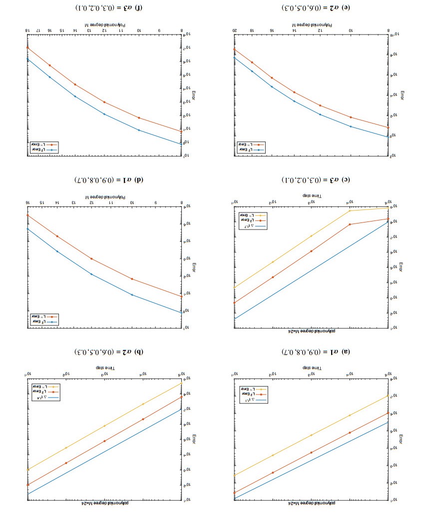
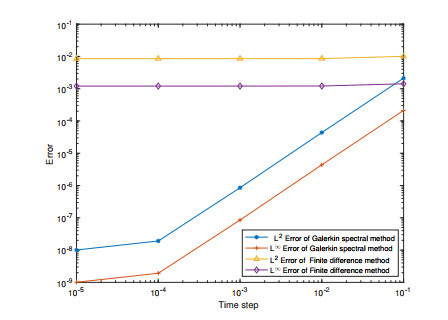
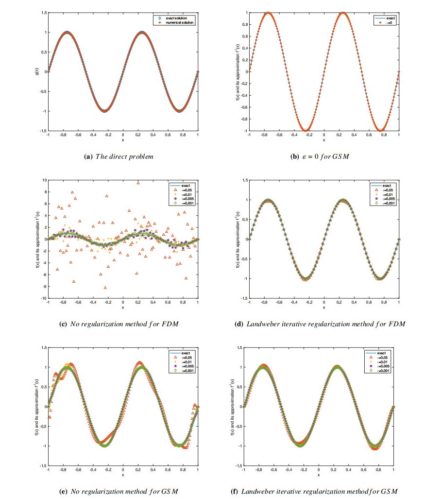
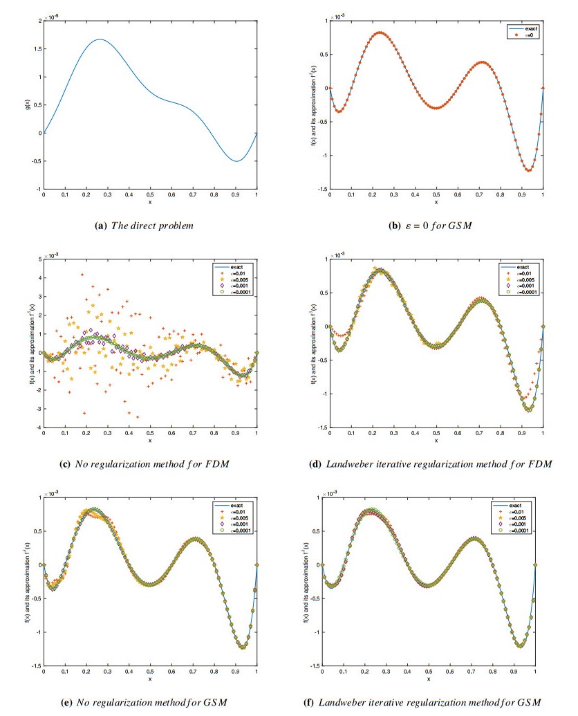
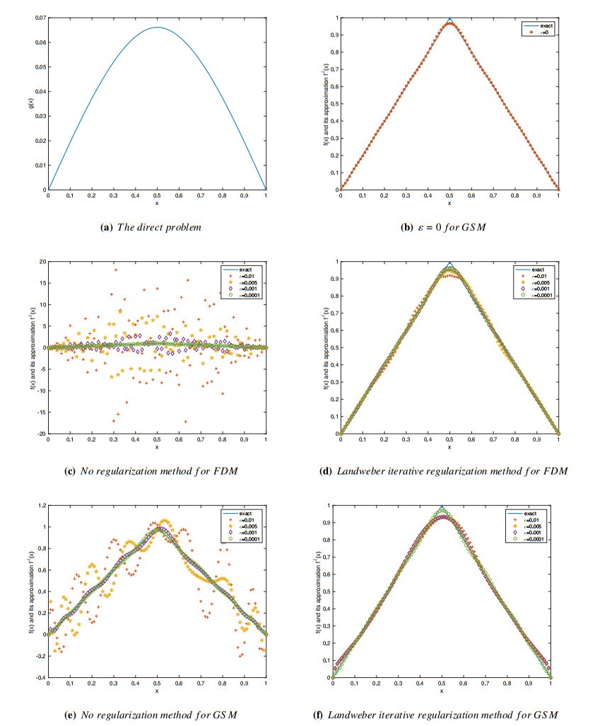
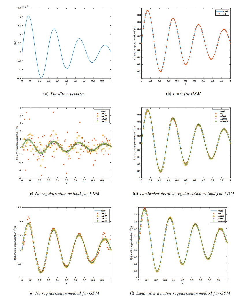
In this paper, we employ the Galerkin spectral method to handle a multi-term time-fractional diffusion equation, and investigate the numerical stability and convergence of the proposed method. In addition, we find an interesting application of the Galerkin spectral method to solving an inverse source problem efficiently from the noisy final data in a general bounded domain, and the uniqueness and the ill-posedness for the inverse problem are proved based on expression of the solution. Furthermore, we compare the calculation results of spectral method and finite difference method without any regularization method, and get a norm estimate of the coefficient matrix of a spectral method discretized. And for that we conclude that the spectral method itself can act as a regularization method for some inverse problem (such as inverse source problem). Finally, several numerical examples are used to illustrate the effectiveness and accuracy of the method.
- Multi-term time-fractional diffusion equation,
- Ill-posed problem,
- Inverse source problem,
- Galerkin spectral method,
- Finite difference method
Citation: L.L. Sun, M.L. Chang. Galerkin spectral method for a multi-term time-fractional diffusion equation and an application to inverse source problem[J]. Networks and Heterogeneous Media, 2023, 18(1): 212-243. doi: 10.3934/nhm.2023008

Related Papers:

Abstract

In this paper, we employ the Galerkin spectral method to handle a multi-term time-fractional diffusion equation, and investigate the numerical stability and convergence of the proposed method. In addition, we find an interesting application of the Galerkin spectral method to solving an inverse source problem efficiently from the noisy final data in a general bounded domain, and the uniqueness and the ill-posedness for the inverse problem are proved based on expression of the solution. Furthermore, we compare the calculation results of spectral method and finite difference method without any regularization method, and get a norm estimate of the coefficient matrix of a spectral method discretized. And for that we conclude that the spectral method itself can act as a regularization method for some inverse problem (such as inverse source problem). Finally, several numerical examples are used to illustrate the effectiveness and accuracy of the method.

References

[1]	R. Metzler, J. Klafter, The random walk's guide to anomalous diffusion: a fractional dynamics approach, Phys. Rev. E, 61 (2000), 6308–6311. https://doi.org/10.1016/s0370-1573(00)00070-3 doi: 10.1016/s0370-1573(00)00070-3
[2]	B. Berkowitz, H. Scher, S. Silliman Anomalous transport in laboratory-scale, heterogeneous porous media, Water Resour. Res., 36 (2000), 149–158. https://doi.org/10.1029/2000wr900026 doi: 10.1029/2000wr900026
[3]	F. Mainardi, Fractional calculus and waves in linear viscoelasticity: an introduction to mathematical models, Singapore: World Scientific, 2010. https://doi.org/10.1142/p614
[4]	Y. Hatano, N. Hatano, Dispersive transport of ions in colum experiments: an explanation of long-tailed profiles, Water Resour. Res., 34 (1998), 1027–1033. https://doi.org/10.1029/98WR00214 doi: 10.1029/98WR00214
[5]	S. Benson, M. B. Meerschaert, Fracral mobile/immobile solute transport, Water Resour. Res., 39 (2003), 1–12. https://doi.org/2003WR002141
[6]	S. Rina, D. A. Benson, M. M. Mark, B. Boris, Fractal mobile/immobile solute transport, Water Resour. Res., 39 (2003), 1296. https://doi.org/10.1029/2003WR002141
[7]	R. R. Nigmatullin, The realization of the generalized transfer equation in a medium with fractal geometry, Phys. Stat. Sol. B, 133 (1986), 425–430. https://doi.org/10.1002/pssb.2221330150 doi: 10.1002/pssb.2221330150
[8]	A. H. Bhrawy, M. A. Zaky, Highly accurate numerical schemes for multi-dimensional space variable-order fractional Schrödinger equations, Comput. Math. Appl., 73 (2017), 1100–1117. https://doi.org/10.1016/j.camwa.2016.11.019 doi: 10.1016/j.camwa.2016.11.019
[9]	Z. Y. Li, Y. K. Liu, M. Yamamoto, Initial-boundary value problems for multi-term time-fractional diffusion equations with positive constant coefficients, Appl. Math. Comput., 257 (2015), 381–397. https://doi.org/10.1016/j.amc.2014.11.073 doi: 10.1016/j.amc.2014.11.073
[10]	Y. Luchko, Initial-boundary-value problems for the generalized multi-term time-fractional diffusion equation, J. Math. Anal. Appl., 374 (2011), 538–548. https://doi.org/10.1016/j.jmaa.2010.08.048 doi: 10.1016/j.jmaa.2010.08.048
[11]	X. L. Ding, J. J. Nieto, Analytical solutions for multi-term time-space fractional partial differential equations with nonlocal damping terms, Fract. Calc. Appl. Anal., 21 (2018), 312–335. https://doi.org/10.1016/j.cnsns.2018.05.022 doi: 10.1016/j.cnsns.2018.05.022
[12]	C. S. Sin, G. I. Ri, M. C. Kim, Analytical solutions to multi-term time-space Caputo-Riesz fractional diffusion equations on an infinite domain, Adv. Difference Equ., 1 (2017), 306. https://doi.org/10.1186/s13662-017-1369-x doi: 10.1186/s13662-017-1369-x
[13]	G. S. Li, C. L. Sun, X. Z. Jia, D. H. Du, Numerical solution to the multi-term time fractional diffusion equation in a finite domain, Numer. Math. Theory Methods Appl., 9 (2016), 337–357. https://doi.org/10.4208/nmtma.2016.y13024 doi: 10.4208/nmtma.2016.y13024
[14]	M. R. Cui, Finite difference schemes for the two-dimensional multi-term time-fractional diffusion equations with variable coefficients, Comput. Appl. Math., 40 (2021), 167. https://doi.org/10.1007/s40314-021-01551-11 doi: 10.1007/s40314-021-01551-11
[15]	Y. L. Zhao, P. Zhu, X. M. Gu, A second-order accurate implicit difference scheme for time fractional reaction-diffusion equation with variable coefficients and time drift term, East Asian J. Appl. Math., 9 (2019), 723–754. https://doi.org/10.4208/eajam.200618.250319 doi: 10.4208/eajam.200618.250319
[16]	Z. Y. Li, O. Y. Imanuvilov, M. Yamamoto, Uniqueness in inverse boundary value problems for fractional diffusion equations, Inverse Problems, 32 (2016), 015004. https://doi.org/10.1088/0266-5611/32/1/015004 doi: 10.1088/0266-5611/32/1/015004
[17]	W. P. Bu, S. Shu, X. Q. Yue, A. G. Xiao, W. Zeng, Space-time finite element method for the multi-term time-space fractional diffusion equation on a two-dimensional domain, Comput. Math. Appl., 75 (2019), 1367–1379. https://doi.org/10.1016/j.camwa.2018.11.033 doi: 10.1016/j.camwa.2018.11.033
[18]	J. Zhou, D. Xu, H. B. Chen, A weak Galerkin finite element method for multi-term time-fractional diffusion equations, East Asian J. Appl. Math., 8 (2018), 181–193. https://doi.org/10.4208/eajam.260617.151117a doi: 10.4208/eajam.260617.151117a
[19]	L. L. Wei, Stability and convergence of a fully discrete local discontinuous Galerkin method for multi-term time fractional diffusion equations, Numer. Algorithms, 76 (2017), 695–707. https://doi.org/10.1007/s11075-017-0277-1 doi: 10.1007/s11075-017-0277-1
[20]	S. M. Guo, L. Q. Mei, Z. Q. Zhang, Y. T. Jiang, Finite difference/spectral-Galerkin method for a two-dimensional distributed-order time-space fractional reaction-diffusion equation, Appl. Math. Lett., 85 (2018), 157–163. https://doi.org/10.1016/j.aml.2018.06.005 doi: 10.1016/j.aml.2018.06.005
[21]	R. M. Zheng, F. W. Liu, X. Y. Jiang, A Legendre spectral method on graded meshes for the two-dimensional multi-term time-fractional diffusion equation with non-smooth solutions, Appl. Math. Lett., 104 (2020), 106247. https://doi.org/10.1016/j.aml.2020.106247 doi: 10.1016/j.aml.2020.106247
[22]	Y. Q. Liu, X. L. Yin, F. W. Liu, X. Y. Xin, Y. F. Shen, L. B. Feng, An alternating direction implicit Legendre spectral method for simulating a 2D multi-term time-fractional Oldroyd-B fluid type diffusion equation, Comput. Math. Appl., 113 (2022), 160–173. https://doi.org/10.1016/j.camwa.2022.03.020 doi: 10.1016/j.camwa.2022.03.020
[23]	M. Zheng, F. Liu, V. Anh, I. Turner, A high-order spectral method for the multi-term time-fractional diffusion equations, Appl. Math. Model., 40 (2016), 4970–4985. https://doi.org/10.1016/j.apm.2015.12.011 doi: 10.1016/j.apm.2015.12.011
[24]	M. A. Zaky, A Legendre spectral quadrature tau method for the multi-term time-fractional diffusion equations, Comput. Appl. Math., 37 (2018), 3525–3538. https://doi.org/10.1007/S40314-017-0530-1 doi: 10.1007/S40314-017-0530-1
[25]	Y. Zhang, X. Xu, Inverse source problem for a fractional diffusion equation, Inverse Probl, 27 (2011), 538–548. https://doi.org/10.1088/0266-5611/27/3/035010 doi: 10.1088/0266-5611/27/3/035010
[26]	T. Wei, L. L. Sun, Y. S. Li, Uniqueness for an inverse space-dependent source term in a multi-dimensional time-fractional diffusion equation, Appl. Math. Lett., 61 (2016), 108–113. https://doi.org/10.1016/j.aml.2016.05.004 doi: 10.1016/j.aml.2016.05.004
[27]	X. B. Yan, T. Wei, Determine a space-dependent source term in a time fractional diffusion-wave equation, Acta Appl. Math., 165 (2020), 163–181. https://doi.org/10.1007/s10440-019-00248-2 doi: 10.1007/s10440-019-00248-2
[28]	L. L. Sun, X. B. Yan, K. Liao, Simultaneous inversion of a fractional order and a space source term in an anomalous diffusion model, J Inverse Ill Posed Probl, 30 (2022), 791–805. https://doi.org/10.1515/jiip-2021-0027 doi: 10.1515/jiip-2021-0027
[29]	S. Yeganeh, R. Mokhtari, J. S. Hesthaven, Space-dependent source determination in a time-fractional diffusion equation using a local discontinuous Galerkin method, BIT Numer. Math., 57 (2017), 685–707. https://doi.org/10.1007/s10543-017-0648-y doi: 10.1007/s10543-017-0648-y
[30]	D. J. Jiang, Z. Y. Li, Y. K. Liu, M. Yamamoto, Weak unique continuation property and a related inverse source problem for time-fractional diffusion-advection equations, Inverse Problems, 33 (2017), 055013. https://doi.org/10.1088/1361-6420/aa58d1 doi: 10.1088/1361-6420/aa58d1
[31]	Y. S. Li, L. L. Sun, Z. Q. Zhang, T. Wei, Identification of the time-dependent source term in a multi-term time-fractional diffusion equation, Numer. Algorithms, 82 (2019), 1279–1301. https://doi.org/10.1007/s11075-019-00654-5 doi: 10.1007/s11075-019-00654-5
[32]	L. L. Sun, X. B. Yan, An inverse source problem for distributed order time-fractional diffusion equation, Adv. Math. Phys., 2020 (2020), 1825235. https://doi.org/10.1155/2020/1825235 doi: 10.1155/2020/1825235
[33]	S. A. Malik, A. Ilyas, A. Samreen, Simultaneous determination of a source term and diffusion concentration for a multi-term space-time fractional diffusion equation, Math. Model. Anal., 26 (2021), 411–431. https://doi.org/10.3846/mma.2021.11911 doi: 10.3846/mma.2021.11911
[34]	L. L. Sun, Y. S. Li, Y. Zhang, Simultaneous inversion of the potential term and the fractional orders in a multi-term time-fractional diffusion equation, Inverse Probl, 37 (2021), 055007. https://doi.org/10.1088/1361-6420/abf162 doi: 10.1088/1361-6420/abf162
[35]	Y. H. Lin, H. Y. Liu, X. Liu, S. Zhang, Simultaneous recoveries for semilinear parabolic systems, Inverse Probl, 38 (2022), 115006. https://doi.org/10.1088/1361-6420/ac91ee doi: 10.1088/1361-6420/ac91ee
[36]	H. Y. Liu, G. Uhlmann, Determining both sound speed and internal source in thermo-and photo-acoustic tomography, Inverse Probl, 31 (2015), 105005. https://doi.org/10.1088/0266-5611/31/10/105005 doi: 10.1088/0266-5611/31/10/105005
[37]	X. L. Cao, H. Y. Liu, Determining a fractional Helmholtz equation with unknown source and scattering potential, Commun. Math. Sci., 17 (2019), 1861–1876. https://doi.org/110.4310/CMS.2019.v17.n7.a5
[38]	L. L. Sun, Y. Zhang, T. Wei, Recovering the time-dependent potential function in a multi-term time-fractional diffusion equation, Appl. Numer. Math., 135 (2019), 228–245. https://doi.org/10.1016/j.apnum.2018.09.001 doi: 10.1016/j.apnum.2018.09.001
[39]	E. Bazhlekova, Properties of the fundamental and the impulse-response solutions of multi-term fractional differential equations, Complex Analysis and Applications, 2 (2013), 55–64.
[40]	C. L. Sun, G. S. Li, X. Z. Jia, Numerical inversion for the initial distribution in the multi-term time-fractional diffusion equation using final observations, Adv. Appl. Math. Mech., 9 (2017), 1525–1546. https://doi.org/10.4208/aamm.OA-2016-0170 doi: 10.4208/aamm.OA-2016-0170
[41]	Y. M. Lin, C. J. Xu, Finite difference/spectral approximations for the time-fractional diffusion equation, J. Comput. Phys., 225 (2007), 1533–1552. https://doi.org/10.1016/j.jcp.2007.02.001 doi: 10.1016/j.jcp.2007.02.001
[42]	C. Bernardi, Y. Maday, Approximations spectrales de problèmes Aux Limites Elliptiques, Paris: Springer-Verlag, 1992.
[43]	K. Sakamoto, M. Yamamoto, Initial value/boundary value problems for fractional diffusion-wave equations and applications to some inverse problems, J. Math. Anal. Appl., 382 (2011), 538–548. https://doi.org/10.1016/j.jmaa.2011.04.058 doi: 10.1016/j.jmaa.2011.04.058
[44]	N. Frank, Regularisierung schlecht gestellter Probleme durch Projektionsverfahren, Numer. Math., 28 (1977), 329–341. https://doi.org/10.1007/BF01389972 doi: 10.1007/BF01389972
[45]	T. Wei, J. G. Wang, A modified quasi-boundary value method for the backward time-fractional diffusion problem, ESAIM Math. Model. Numer. Anal., 48 (2014), 603–621. https://doi.org/10.1051/m2an/2013107 doi: 10.1051/m2an/2013107

Reader Comments

Your name:*

Email:*
© 2023 the Author(s), licensee AIMS Press. This is an open access article distributed under the terms of the Creative Commons Attribution License (http://creativecommons.org/licenses/by/4.0)