Assessment of serum interleukin 19 level in patients with warts

Radwa El-Sayed Mahmoud Marie; Aya Mohamed kamal Lasheen; Hebat-Allah Hassan Nashaat; Mona A. Atwa; Radwa El-Sayed Mahmoud Marie; Aya Mohamed kamal Lasheen; Hebat-Allah Hassan Nashaat; Mona A. Atwa

doi:10.3934/molsci.2023001

AIMS Molecular Science

2023, Volume 10, Issue 1: 1-10. doi: 10.3934/molsci.2023001

Previous Article Next Article

Research article

Assessment of serum interleukin 19 level in patients with warts

1.
Department of Dermatology, Venereology and Andrology, Faculty of Medicine, Suez Canal University, Ismailia, Egypt
2.
Department of Dermatology, Ministry of Health and Population, Damietta Hospital for Dermatology and Leprosy, Damietta, Egypt
3.
Department of Clinical Pathology, Faculty of Medicine, Suez Canal University, Ismailia, Egypt

Received: 13 September 2022 Revised: 08 December 2022 Accepted: 20 December 2022 Published: 12 January 2023

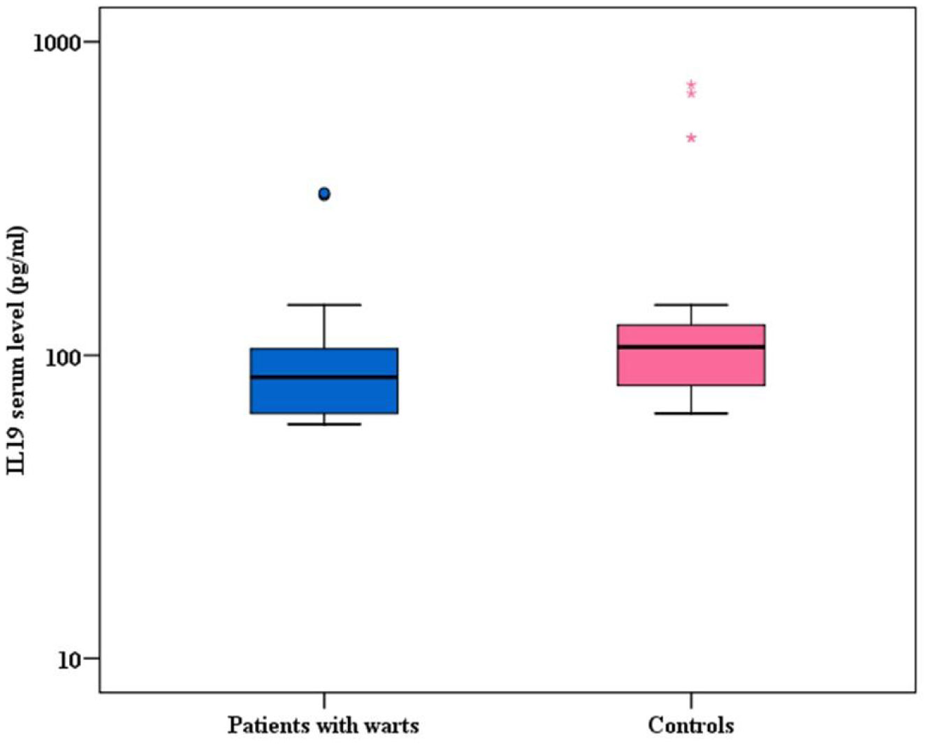
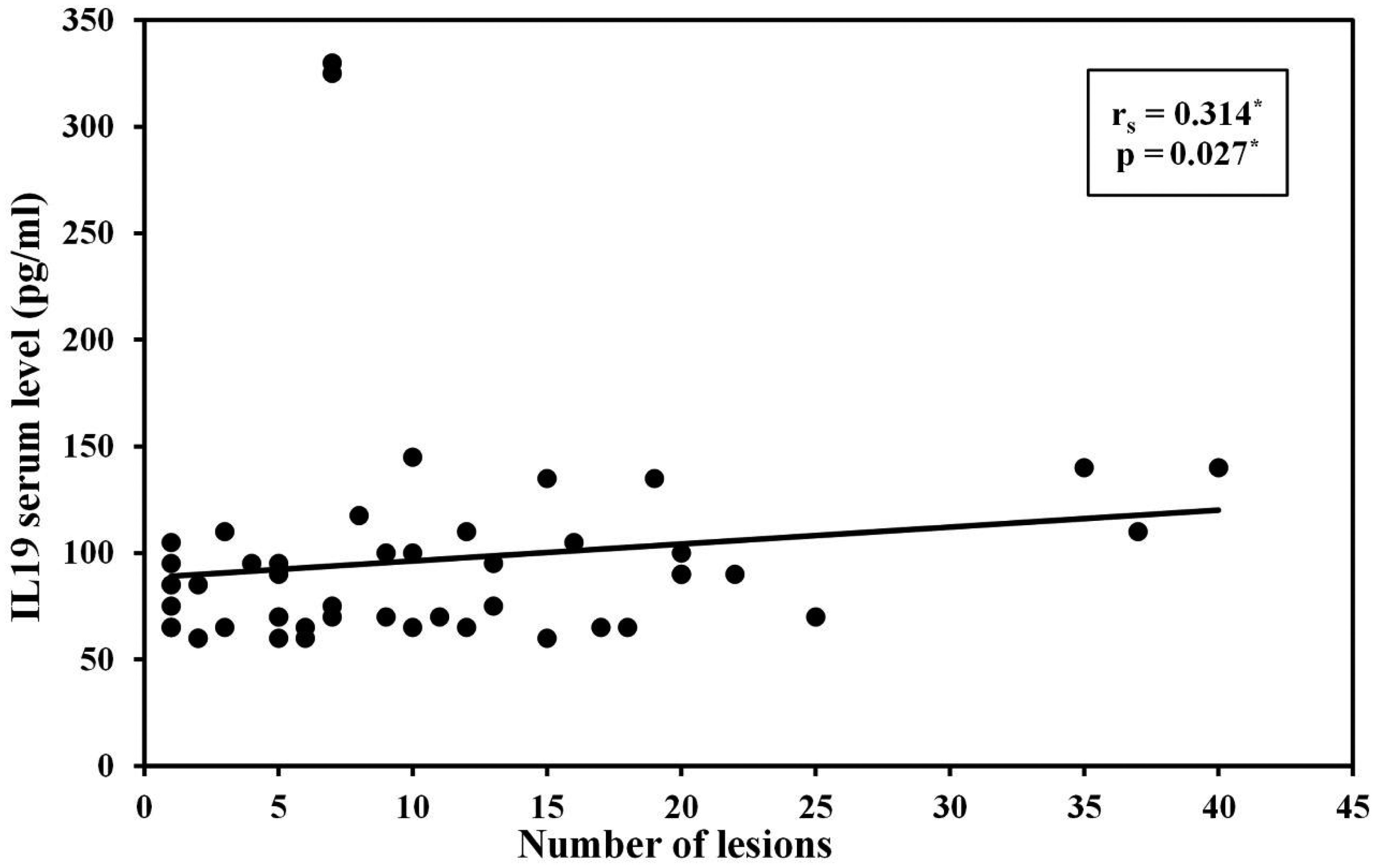
Background: Warts are viral cutaneous infections caused by human papilloma virus (HPV), presented by verrucous growth over the skin surface. The cell mediated immune response is considered to play a crucial role in HPV clearance. The viral load and number of lesions increase when there is an imbalance between the T-helper 1 and T-helper 2 immune responses. Interleukin (IL)-19 is a cytokine that belongs to interleukin 10 cytokines family and constitutes a sub-family with IL-20, IL-22 and IL-24. IL-19 is mainly produced by activated monocytes and to a lesser extent by B-cells, keratinocytes and fetal membranes. IL-19 was found to shift T-cell maturation away from the pro-inflammatory T-helper 1 cells toward the anti-inflammatory T-helper 2 cells. It induces IL-4 and IL-13 production in T cells and apoptosis in monocytes. Aim: This study aimed to measure serum level of IL-19 in patients with warts compared to healthy controls and to find out the correlation between this level and number, size and clinical types of warts. Methods: The study included 50 patients with warts and 50 control subjects. Serum concentration of IL-19 was measured by enzyme-linked immune sorbent assay. Results: Interleukin-19 serum level was significantly lower in patients with warts than in controls (P < 0.003). Moreover, there was a significant positive correlation between IL-19 serum level and the number of warts (P = 0.027). Conclusion: Serum level of IL-19 was significantly lower in patients with warts, and this low level might be crucial for an effective cell mediated immunological response to HPV.
- wart,
- infection,
- interleukin-19,
- human papilloma virus,
- immunological response
Citation: Radwa El-Sayed Mahmoud Marie, Aya Mohamed kamal Lasheen, Hebat-Allah Hassan Nashaat, Mona A. Atwa. Assessment of serum interleukin 19 level in patients with warts[J]. AIMS Molecular Science, 2023, 10(1): 1-10. doi: 10.3934/molsci.2023001

Related Papers:

Abstract

Background: Warts are viral cutaneous infections caused by human papilloma virus (HPV), presented by verrucous growth over the skin surface. The cell mediated immune response is considered to play a crucial role in HPV clearance. The viral load and number of lesions increase when there is an imbalance between the T-helper 1 and T-helper 2 immune responses. Interleukin (IL)-19 is a cytokine that belongs to interleukin 10 cytokines family and constitutes a sub-family with IL-20, IL-22 and IL-24. IL-19 is mainly produced by activated monocytes and to a lesser extent by B-cells, keratinocytes and fetal membranes. IL-19 was found to shift T-cell maturation away from the pro-inflammatory T-helper 1 cells toward the anti-inflammatory T-helper 2 cells. It induces IL-4 and IL-13 production in T cells and apoptosis in monocytes. Aim: This study aimed to measure serum level of IL-19 in patients with warts compared to healthy controls and to find out the correlation between this level and number, size and clinical types of warts. Methods: The study included 50 patients with warts and 50 control subjects. Serum concentration of IL-19 was measured by enzyme-linked immune sorbent assay. Results: Interleukin-19 serum level was significantly lower in patients with warts than in controls (P < 0.003). Moreover, there was a significant positive correlation between IL-19 serum level and the number of warts (P = 0.027). Conclusion: Serum level of IL-19 was significantly lower in patients with warts, and this low level might be crucial for an effective cell mediated immunological response to HPV.

Abbreviations

Interleukin

HPV

Human papilloma virus

T-helper

ELISA

Enzyme-Linked Immune-sorbent Assay

HRP

Horseradish Peroxidase

optical density

HBV

Hepatitis B virus

Conflicts of Interest

All authors declare no conflicts of interest in this paper.

References

[1]	Paaso A, Koskimaa HM, Welters MJ, et al. (2015) Cell mediated immunity against HPV16 E2, E6 and E7 peptides in women with incident CIN and in constantly HPV-negative women followed-up for 10-years. J Transl Med 13: 1-11. https://doi.org/10.1186/s12967-015-0498-9
[2]	Steinbach A, Riemer AB (2018) Immune evasion mechanisms of human papillomavirus. Int J Cancer 142: 224-229. https://doi.org/10.1002/ijc.31027
[3]	Fujimoto Y, Azuma YT, Matsuo Y, et al. (2017) Interleukin-19 contributes as a protective factor in experimental Th2-mediated colitis. Naunyn. Schmiedebergs. Arch Pharmacol 390: 261-268. https://doi.org/10.1007/s00210-016-1329-0
[4]	Sabat R (2010) IL-10 family of cytokines. Cytokine Growth Factor Rev 21: 315-324. https://doi.org/10.1016/j.cytogfr.2010.11.001
[5]	Gallagher G, Eskdale J, Jordan W, et al. (2004) Human interleukin-19 and its receptor: a potential role in the induction of Th2 responses. Int Immunopharmacol 4: 615-626. https://doi.org/10.1016/j.intimp.2004.01.005
[6]	Schiffman M, Doorbar J, Wentzensen N, et al. (2016) Carcinogenic human papillomavirus infection. Nat Rev Dis Primers 2: 16086. https://doi.org/10.1038/nrdp.2016.86
[7]	Fernandes JV, DE Medeiros Fernandes TA, DE Azevedo JC, et al. (2015) Link between chronic inflammation and human papillomavirus-induced carcinogenesis (Review). Oncol Lett 9: 1015-1026. https://doi.org/10.3892/ol.2015.2884
[8]	Liao SC, Cheng YC, Wang YC, et al. (2004) IL-19 induced Th2 cytokines and was up-regulated in asthma patients. J Immunol 173: 6712-6718. https://doi.org/10.4049/jimmunol.173.11.6712
[9]	Oguejiofor K, Hall J, Slater C, et al. (2015) Stromal infiltration of CD8 T cells is associated with improved clinical outcome in HPV-positive oropharyngeal squamous carcinoma. Br J Cancer 113: 886-893. https://doi.org/10.1038/bjc.2015.277
[10]	Azuma YT, Nishiyama K (2020) Interleukin-19 enhances cytokine production induced by lipopolysaccharide and inhibits cytokine production induced by polyI:C in BALB/c mice. J Vet Med Sc 82: 891-896. https://doi.org/10.1292/jvms.20-0137
[11]	Liao YC, Liang WG, Chen FW, et al. (2002) IL-19 induces production of IL-6 and TNF-alpha and results in cell apoptosis through TNF-alpha. J Immunol 169: 4288-4297. https://doi.org/10.4049/jimmunol.169.8.4288
[12]	Hsu YH, Li HH, Sung JM, et al. (2013) Interleukin-19 mediates tissue damage in murine ischemic acute kidney injury. PLoS One 8: e56028. https://doi.org/10.1371/journal.pone.0056028
[13]	AH, Esawy AM, Khalifa NA, et al. (2020) Evaluation of serum interleukin 17 and zinc levels in recalcitrant viral wart. J Cosmet Dermatol 19: 954-959. https://doi.org/10.1111/jocd.13106
[14]	Xu X, Prens E, Florencia E, et al. (2021) Interleukin-17A Drives IL-19 and IL-24 Expression in Skin Stromal Cells Regulating Keratinocyte Proliferation. Front Immunol 12: 719562. https://doi.org/10.3389/fimmu.2021.719562
[15]	Wang Y, Liu X, Li Y, et al. (2013) The paradox of IL-10-mediated modulation in cervical cancer (Review). Biomedical Reports 1: 347-351. https://doi.org/10.3892/br.2013.69
[16]	Berti FCB, Pereira APL, Cebinelli GCM, et al. (2017) The role of interleukin 10 in human papilloma virus infection and progression to cervical carcinoma. Cytokine Growth Factor Rev 34: 1-13. https://doi.org/10.1016/j.cytogfr.2017.03.002
[17]	Marie REM, Abuzeid AQEM, Attia FM, et al. (2021) Serum level of interleukin-22 in patients with cutaneous warts: A case-control study. J Cosmet Dermatol 2021: 1782-1787. https://doi.org/10.1111/jocd.13779

Reader Comments

Your name:*

Email:*
© 2023 the Author(s), licensee AIMS Press. This is an open access article distributed under the terms of the Creative Commons Attribution License (http://creativecommons.org/licenses/by/4.0)