<i>d</i>-Limonene challenging anti-inflammatory strategies

Patrizia A d'Alessio; Marie C Béné; Chantal Menut; Patrizia A d'Alessio; Marie C Béné; Chantal Menut

doi:10.3934/molsci.2022003

AIMS Molecular Science

2022, Volume 9, Issue 2: 46-65. doi: 10.3934/molsci.2022003

Previous Article Next Article

Research article

d-Limonene challenging anti-inflammatory strategies

1.
AISA Therapeutics, University Paris Sud-11 and Genopole, Evry, France
2.
Hematology Biology, CHU de Nantes & Inserm 1232 CRCINA, Nantes, France
3.
IBMM, Univ Montpellier, CNRS, ENSCM, Montpellier, France

Received: 12 November 2021 Revised: 09 January 2022 Accepted: 07 April 2022 Published: 20 April 2022

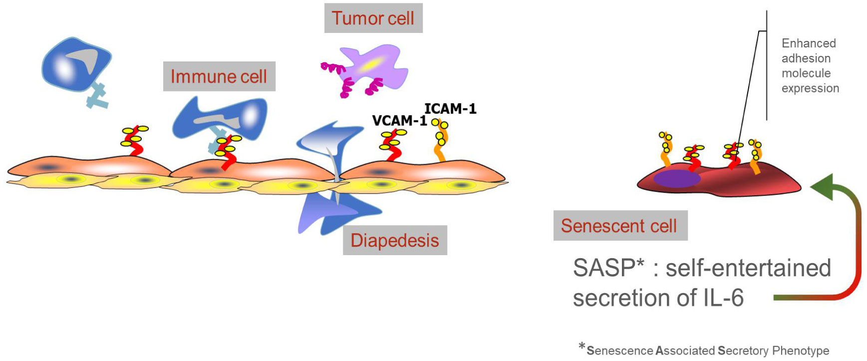
Aging and senescence seem linked by fundamental, yet still ill-understood mechanisms. For this reason, this paper expands on the background of a discovery that still has to gain acknowledgement by public policies to find its place in a market hungry for a non-toxic anti-inflammatory molecule. Reversibility of the senescent cell phenotype was the starting-point of a research that turned out to identify the monoterpenes class of molecules as able to achieve this goal. Indeed, these compounds strongly inhibit the circulation of pro-inflammatory cytokines as well as the expression of cell-anchored adhesive molecules, liable to recruit activated immune cells. Starting from cell-based studies, the pre-clinical and clinical assays reported here confirmed the capacities of these compounds, both in experimental colitis, dermatitis and stress murine models, but also in-human studies addressing the latent chronic inflammation associated with age or psoriasis. Last but not least, because of an intriguing mechanism yet not totally unraveled and most probably depending on the effect of monoterpenes on gut microbiota strains–apart from assuring a constant gut barrier repair-a consistent Quality of Life amelioration, i.e. mood modulation probably due to enhanced dopamine secretion was also demonstrated. Finally, after entering in more pharmacologic considerations on toxicity and bio-availability studies as for the safety of this class of compounds, a strategic positioning of the precious role of anti-inflammatory drugs in a market that has yet to overcome common chronic diseases because of their predisposing condition not only to cancer and neuro-degenerative diseases but now also to COVID-19 is envisioned.
- drug discovery,
- anti-inflammatory molecules,
- monoterpenes,
- d-Limonene,
- common chronic diseases,
- aging,
- cell senescence
Citation: Patrizia A d'Alessio, Marie C Béné, Chantal Menut. d-Limonene challenging anti-inflammatory strategies[J]. AIMS Molecular Science, 2022, 9(2): 46-65. doi: 10.3934/molsci.2022003

Related Papers:

Abstract

Aging and senescence seem linked by fundamental, yet still ill-understood mechanisms. For this reason, this paper expands on the background of a discovery that still has to gain acknowledgement by public policies to find its place in a market hungry for a non-toxic anti-inflammatory molecule. Reversibility of the senescent cell phenotype was the starting-point of a research that turned out to identify the monoterpenes class of molecules as able to achieve this goal. Indeed, these compounds strongly inhibit the circulation of pro-inflammatory cytokines as well as the expression of cell-anchored adhesive molecules, liable to recruit activated immune cells. Starting from cell-based studies, the pre-clinical and clinical assays reported here confirmed the capacities of these compounds, both in experimental colitis, dermatitis and stress murine models, but also in-human studies addressing the latent chronic inflammation associated with age or psoriasis. Last but not least, because of an intriguing mechanism yet not totally unraveled and most probably depending on the effect of monoterpenes on gut microbiota strains–apart from assuring a constant gut barrier repair-a consistent Quality of Life amelioration, i.e. mood modulation probably due to enhanced dopamine secretion was also demonstrated. Finally, after entering in more pharmacologic considerations on toxicity and bio-availability studies as for the safety of this class of compounds, a strategic positioning of the precious role of anti-inflammatory drugs in a market that has yet to overcome common chronic diseases because of their predisposing condition not only to cancer and neuro-degenerative diseases but now also to COVID-19 is envisioned.

References

[1]	Califf RM (2021) Avoiding the coming tsunami of common, chronic disease: what the lessons of the COVID-19 pandemic can teach us. Circulation 143: 1831-1834. https://doi.org/10.1161/CIRCULATIONAHA.121.053461
[2]	Horton R (2020) Covid-19 is not a pandemic. Lancet 396: 874. https://doi.org/10.1016/S0140-6736(20)32000-6
[3]	Proshkina E, Plyusnin S, Babak T, et al. (2020) Terpenoids as potential geroprotectors. Antioxidants (Basel) 9: 529. https://doi.org/10.3390/antiox9060529
[4]	Quintans JSS, Shanmugam S, Heimfarth L, et al. (2019) Monoterpenes modulating cytokines - A review. Food Chem Toxicol 123: 233-257. https://doi.org/10.1016/j.fct.2018.10.058
[5]	Horton R (1996) Vioxx, the implosion of Merck, and aftershocks at the FDA. Lancet 364: 1995-1996. https://doi.org/10.1016/S0140-6736(04)17523-5
[6]	Topol EJ (2004) Failing the public health-rofeoxib, Merck, and the FDA. N Engl J Med 351: 1707-1709. https://doi.org/10.1056/NEJMp048286
[7]	d'Alessio PA, Béné MC (2020) AISA can control the inflammatory facet of SASP. Mech Ageing Dev 186: 111206. https://doi.org/10.1016/j.mad.2019.111206
[8]	d'Alessio PA, Dhombres J (2005) Architecture of life, from Plato to tensegrity. Science et Technique en Perspective 9.Brepols éds.
[9]	Laberge RM, Zhou L, Sarantos MR, et al. (2012) Glucocorticoids suppress selected components of the senescence-associated secretory phenotype. Aging Cell 11: 569-578. https://doi.org/10.1111/j.1474-9726.2012.00818.x
[10]	Crowell PL, Lin S, Vedejs E, Gould MN (1992) Identification of metabolites of the antitumor agent d-Limonene capable of inhibiting protein isoprenylation and cell growth. Cancer Chemother Pharmacol 31: 205-212. https://doi.org/10.1007/BF00685549
[11]	Crowell PL, Elson CE, Bailey HH, et al. (1994) Human metabolism of the experimental cancer therapeutic agent d-Limonene. Cancer Chemother Pharmacol 35: 31-37. https://doi.org/10.1007/BF00686281
[12]	d'Alessio PA, Ostan R, Bisson JF, et al. (2013) Oral administration of d-limonene controls inflammation in rat colitis and displays anti-inflammatory properties as diet supplementation in humans. Life Sci 92: 1151-1156. https://doi.org/10.1016/j.lfs.2013.04.013
[13]	Ruszkowski J, Daca A, Szewczyk A, et al. (2021) The influence of biologics on the microbiome in immune-mediated inflammatory diseases: A systematic review. Biomed Pharmacother 141: 111904. https://doi.org/10.1016/j.biopha.2021.111904
[14]	Reis G, Dos Santos Moreira-Silva EA, Medeiros Silva DC, et al. (2021) Effect of early treatment with fluvoxamine on risk of emergency care and hospitalisation among patients with COVID-19: the TOGETHER randomised, platform clinical trial. Lancet Glob Health : S2214-109X(21)00448–4.
[15]	Winthrop KL, Skolnick AW, Rafiq AM, et al. Opaganib in COVID-19 pneumonia: Results of a randomized, placebo-controlled Phase 2a trial (2021). https://doi.org/10.1101/2021.08.23.21262464
[16]	Simonsen JL (1947) The Terpenes vol. Cambridge: In University Press 143-165.
[17]	Bakkali F, Averbeck S, Averbeck D, et al. (2008) Biological effects of essential oils-a review. Food Chem Toxicol 46: 446-475. https://doi.org/10.1016/j.fct.2007.09.106
[18]	Gualdani R, Cavalluzzi MM, Lentini G, et al. (2016) The chemistry and pharmacology of citrus limonoids. Molecules 21: E1530. https://doi.org/10.3390/molecules21111530
[19]	Pultrini Ade M, Galindo LA, Costa M (2006) Effects of the essential oil from Citrus aurantium L. in experimental anxiety models in mice. Life Sci 78: 1720-1725. https://doi.org/10.1016/j.lfs.2005.08.004
[20]	d'Alessio P. (2000) Endothelium as pharmacological target. Curr Op Invest Drugs 2: 1720-1724.
[21]	Golias C, Tsoutsi E, Matziridis A, et al. (2007) Leukocyte and endothelial cell adhesion molecules in inflammation focusing on inflammatory heart disease. In Vivo 21: 757-769.
[22]	Schnoor M (2015) Endothelial actin-binding proteins and actin dynamics in leukocyte transendothelial migration. J Immunol 194: 3535-3541. https://doi.org/10.4049/jimmunol.1403250
[23]	Coppé JP, Desprez PY, Krtolica A, Campisi J, et al. (2010) The senescence-associated secretory phenotype: the dark side of tumor suppression. Annu Rev Pathol 5: 99-118. https://doi.org/10.1146/annurev-pathol-121808-102144
[24]	Franceschi C, Campisi J (2014) Chronic inflammation (inflammaging) and its potential contribution to age-associated diseases. J Gerontol A Biol Sci Med Sci 69: S4-S9. https://doi.org/10.1093/gerona/glu057
[25]	Chaudière J, Moutet M, d'Alessio P (1995) Antioxidant and anti-inflammatory protection of vascular endothelial cells by new synthetic mimics of glutathione peroxidase. CR Seances Soc Biol Fil 189: 861-882.
[26]	D'Anna R, Le Buanec H, Alessandri G, et al. (2001) Selective activation of cervical microvascular endothelial cells by human papillomavirus 16-e7 oncoprotein. J Natl Cancer Inst 93: 1843-1851. https://doi.org/10.1093/jnci/93.24.1843
[27]	d'Alessio P (2004) Aging and the endothelium. Exp Gerontol 39: 165-171. https://doi.org/10.1016/j.exger.2003.10.025
[28]	Edelman GM (1993) A golden age for adhesion. Cell Adhes Commun 1: 1-7. https://doi.org/10.3109/15419069309095677
[29]	Ingber D E, Jamieson JD (1985) Cells as tensegrity structures: architectural regulation of histodifferentiation by physical forces transduced over basement membrane. In Gene Expression During Normal and Malignant Differentiation. Orlando, Florida: Academic Press 13-32.
[30]	Wang N, Naruse K, Stamenović D, Fredberg JJ, et al. (2001) Mechanical behavior in living cells consistent with the tensegrity model. Proc Natl Acad Sci USA 98: 7765-7770. https://doi.org/10.1073/pnas.141199598
[31]	(2009) Handbook of Essential OilsScience, Technology and Applications by K. Hüsnü Can Başer and Gerhard Buchbauer Eds. CRC Press: Boca Raton, FL, USA.
[32]	Bisson JF, Menut C, d'Alessio P (2008) Anti-inflammatory senescence actives 5203-L molecule to promote healthy aging and prolongation of lifespan. Rejuvenation Res 11: 399-407. https://doi.org/10.1089/rej.2008.0667
[33]	Bayly MJ, Holmes GD, Forster PI, et al. (2013) Major clades of Australasian Rutoideae (Rutaceae) based on rbcL and atpB sequences. PLoS One 8: e72493. https://doi.org/10.1371/journal.pone.0072493
[34]	d'Alessio PA Composition for treating or preventing cell degeneration using at least one molecule capable of maintaining adhesion molecule expression reversibility and vascular endothelium actin fibre polymerization. Granted in Europe (EP 1 748 771) & US (US-2009-0012162).
[35]	Stayrook KR, McKinzie JH, Barbhaiya LH, et al. (1998) Effects of the anti-tumoragent perillyl alcohol on H-Ras vs. K-Ras farnesylation and signal transduction in pancreatic cells. Anticancer Res 18: 823-828.
[36]	Crowell PL, Siar Ayoubi A, Burke YD (1996) Antitumorigenic effects of limonene and perillyl alcohol against pancreatic and breast cancer. Adv Exp Med Biol 401: 131-136. https://doi.org/10.1007/978-1-4613-0399-2_10
[37]	Toussaint O, Dumont P, Dierick JF, et al. (2000) Stress-induced premature senescence. Essence of life, evolution, stress, and aging. Ann N Y Acad Sci 908: 85-98. https://doi.org/10.1111/j.1749-6632.2000.tb06638.x
[38]	Franceschi C, Bonafè M, Valensin S, et al. (2000) Inflamm-aging. An evolutionary perspective on immunosenescence. Ann N Y Acad Sci 908: 244-254. https://doi.org/10.1111/j.1749-6632.2000.tb06651.x
[39]	Wang N, Butler JP, Ingber DE (1993) Mechanotransduction across the cell surface and through the cytoskeleton. Science 260: 1124-1127. https://doi.org/10.1126/science.7684161
[40]	d'Alessio PA, Mirshahi M, Bisson JF, et al. (2014) Skin repair properties of d-Limonene and perillyl alcohol in murine models. Antiinflamm Antiallergy Agents Med Chem 13: 29-35. https://doi.org/10.2174/18715230113126660021
[41]	König J, Wells J, Cani PD, et al. (2016) Human intestinal barrier function in health and disease. Clin Transl Gastroenterol 7: e196. https://doi.org/10.1038/ctg.2016.54
[42]	d'Alessio PA, Bisson JF, Béné MC (2014) Anti-stress effects of d-Limonene and its metabolite perillyl alcohol. Rejuvenation Res 17: 145-149. https://doi.org/10.1089/rej.2013.1515
[43]	Toussaint O, Dumont P, Remacle J, et al. (2002) Stress-induced premature senescence or stress-induced senescence-like phenotype: one in vivo reality, two possible definitions?. Sci World J 2: 230-247. https://doi.org/10.1100/tsw.2002.100
[44]	Fukumoto S, Sawasaki E, Okuyama S, et al. (2006) Flavor components of monoterpenes in citrus essential oils enhance the release of monoamines from rat brain slices. Nutr Neurosci 9: 73-80. https://doi.org/10.1080/10284150600573660
[45]	Ostan R, Béné MC, Spazzafumo L, et al. (2016) Impact of diet and nutraceutical supplementation on inflammation in elderly people. Results from the RISTOMED study, an open-label randomized control trial. Clin Nutr 35: 812-818. https://doi.org/10.1016/j.clnu.2015.06.010
[46]	Rossi A, Béné MC, Carlesimo M, et al. (2015) Efficacy of orange peel extract in psoriasis. Glob J Dermatol Venereology 3: 1-4. https://doi.org/10.12970/2310-998X.2015.03.01.1
[47]	Bohlmann J, Meyer-Gauen G, Croteau R (1998) Plant terpenoid synthases: molecular biology and phylogenetic analysis. Proc Natl Acad Sci USA 95: 4126-4133. https://doi.org/10.1073/pnas.95.8.4126
[48]	Chen H, Chan KK, Budd T (1998) Pharmacokinetics of d-Limonene in the rat by GC-MS assay. J Pharm Biomed Analysis 17: 631-640. https://doi.org/10.1016/S0731-7085(97)00243-4
[49]	Igim H, Nishimura M, Kodoma R, et al. (1974) Studies on the metabolism of d-Limonene in rats. Xenobiotica 4: 77-84. https://doi.org/10.3109/00498257409049347
[50]	Hardcastle IR, Rowlands MG, Barber AM, et al. (1999) Inhibition of protein prenylation by metabolites of d-Limonene. Biochem Pharmacol 57: 801-809. https://doi.org/10.1016/S0006-2952(98)00349-9
[51]	Vigushin DM, Poon GK, Boddy A, et al. (1998) Phase I and pharmacokinetic study of D-limonene in patients with advanced cancer. Cancer Research Campaign Phase I/II Clinical Trials Committee. Cancer Chemother Pharmacol 42: 111-117. https://doi.org/10.1007/s002800050793
[52]	Hudes GR, Szarka CE, Adams A, et al. (2000) Phase I pharmacokinetic trial of perillyl alcohol (NSC 641066) in patients with refractory solid malignancies. Clin Cancer Res 6: 3071-3080.
[53]	Sun J. D (2007) Limonene: safety and clinical applications. Altern Med Rev 12: 259-264.
[54]	Schnuch A, Uter W, Geier J, et al. (2007) Sensitization to 26 fragrances to be labeled according to current European regulation. Results of the IVDK and review of the literature. Contact Dermatitis 57: 1-10. https://doi.org/10.1111/j.1600-0536.2007.01088.x
[55]	Grief N (1967) Cutaneous safety of fragrance material as measured by the maximisation test. Amer Perfumer Cosmetics 82: 54-57.
[56]	Karlberg AT, Dooms-Goossens A (1997) Contact allergy to oxidized d-limonene among dermatitis patients. Contact Dermatitis 36: 201-206. https://doi.org/10.1111/j.1600-0536.1997.tb00270.x
[57]	Bråred Christensson J, Andersen KE, Bruze M, et al. (2013) An international multicentre study on the allergenic activity of air-oxidized R-limonene. Contact Dermatitis 68: 214-223. https://doi.org/10.1111/cod.12036
[58]	Pesonen M, Suomela S, Kuuliala O, et al. (2014) Occupational contact dermatitis caused by D-limonene. Contact Dermatitis 71: 273-279. https://doi.org/10.1111/cod.12287
[59]	Audrain H, Kenward C, Lovell CR, et al. (2014) Allergy to oxidized limonene and linalool is frequent in the U.K. Br J Dermatol 171: 292-297. https://doi.org/10.1111/bjd.13037
[60]	Shimada T, Shindo M, Miyazawa M (2002) Species differences in the metabolism of (+)- and (-) Limonenes and their metabolites, carveols and carvones, by cytochrome P450 enzymes in liver microsomes of mice, rats, guinea pigs, rabbits, dogs, monkeys, and humans. Drug Metabol Pharmacokin 17: 507-515. https://doi.org/10.2133/dmpk.17.507
[61]	Powers KA, Hooser SB, Sundberg JP, et al. (1998) An evaluation of the acute toxicity of an insecticidal spray containing linalool, d-Limonene, and piperonyl butoxide applied topically to domestic cats. Vet Hum Toxicol 30: 206-210.
[62]	Hooser SB, Beasley VR, Everitt JI (1986) Effects of an insecticidal dip containing d-Limonene in the cat. J Am Vet Med Assoc 189: 905-908.
[63]	Hink WF, Fee BJ (1986) Toxicity of d-Limonene, the major component of citrus peel oil, to all life stages of the cat flea, Ctenocephalides felis (Siphonaptera: pulicidae). J Med Entomol 23: 400-404. https://doi.org/10.1093/jmedent/23.4.400
[64]	Sarkar A, Lehto SM, Harty S, et al. (2016) Psychobiotics and the manipulation of bacteria-gut-brain signals. Trends Neurosci 39: 763-781. https://doi.org/10.1016/j.tins.2016.09.002

Reader Comments

Your name:*

Email:*
© 2022 the Author(s), licensee AIMS Press. This is an open access article distributed under the terms of the Creative Commons Attribution License (http://creativecommons.org/licenses/by/4.0)