Wind-blown particulate transport: A review of computational fluid dynamics models

List of main symbols

1.   Introduction

Particle transport by the wind is a phenomenon of interest for civil engineering projects, environmental problems, and industrial applications.

In fact, transport and consequent deposition of snow and sand on streets, railways, highways, roofs, and buildings can cause serious problems in terms of operation conditions and damages. Similarly, heavy rainfall and hail can cause discomfort and damages as well. The main interest of this review is in dealing with such atmospheric agents that present similar physical transport mechanisms. On the other hand, we will not deal with air pollutants typically characterized by much smaller dimensions. In fact, though their dispersion mechanisms might share some similarities, they also present major differences. Looking at the phenomena involved in the transport of particulate materials lying on the ground, such as sand and snow, one can observe that a crucial mechanism is their lift-off from the ground. Different phenomena contribute to it and their relevance mainly depends on two factors: particle size and wind velocity profile close to the ground.

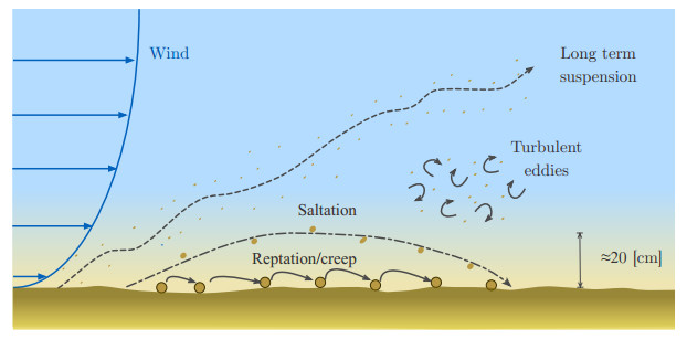
This triggering transport mechanism, named saltation ^[63], is a phenomenon that takes place if the wall shear stress $\tau$ on the ground surface generated by the blowing wind exceeds a threshold value $\tau_t$. This threshold value strongly depends on particles properties such as size and on chemical interactions among them, in conjunction with environmental conditions such as humidity, size and wetting. As reported in ^[50], it is also affected by the local slope of the ground surface.

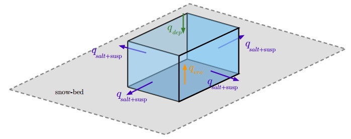
Referring to Figure 1, after lifting-off, the smallest particles are entrained in the wind flow and remain in suspension for a long period. On the other hand, bigger particles, whose aerodynamic behavior is also strongly affected by their shape, follow ballistic trajectories before impacting again on the ground, transferring momentum to other particles which are then ejected from the soil. In this way saltating particles are also able to displace particles that are too heavy to lift-off, and induce very short trajectories that trigger a transport phenomenon called reptation (mainly occurring in sand transport). Another process involving big particles is creep, that consists in particle rolling and sliding on the surface made of other deposited particles.

Erosion and subsequent sedimentation of particles on the ground determine the evolution of the ground surface. This fact makes the mathematical problem a free-boundary value problem. In cases that are severe for snow but not so severe for sand, the particles on the surface slide down forming avalanches, that also contribute to the shaping of the surface of the sedimented particulate.

The quantification of such phenomena suffers from the difficulties in performing experiments both in controlled environments and in-situ. In fact, from the experimental point of view, the presence of particles in the air and the need to monitor and measure their properties make wind tunnel experiments more difficult and onerous. Such kinds of tests have been performed mainly for sand, snow, and rain (see for instance ^{[56,57,58,104,119]}). However, in-situ measurements can be very expensive and time consuming as well. So, even though experiments are fundamental to shed light on the physical phenomena involved, nowadays they are more and more supported by computational simulations, because they are characterized by a high flexibility and can provide affordable results. In fact, thanks to significant improvements in terms of computational performance obtained in the last decade and to the continuous development of new mathematical models, computational simulations have become a catchy tool for all the people interested in these processes and in particular in testing civil and industrial applications. The interest is confirmed by the trend of integrating the dynamics of sand, snow, and rain in Computational Fluid Dynamics (CFD) commercial codes. Some examples of such CFD approaches are listed in ^[107] for snow and ^[17] for rain.

As usual, in dealing with phenomena involving many different phenomena a balance between modelling accuracy and simplicity is required and the choice mainly depends on the level of detail required by the specific application. In fact, on the one hand using over-simplified models may lead to unsatisfactory results compared to experimental data, though in particular situations they might show a qualitative agreement with the real natural phenomenon of interest. On the other hand, including more details leads to an increase of the complexity of the model, and consequently of the computational cost. In this respect, starting from the engineering needs of modeling the fall and transport of snow, sand, and rain, the aim of this review is then to describe and classify the different modelling approaches that have been proposed in the literature possibly mentioning their advantages and disadvantages.

The fundamental requirement of models dealing with particulate transport is their ability to accurately treat the wind dynamics in a very high Reynolds number regime and in a domain characterized by the presence of bluff bodies, like obstacles and infrastructures in general. Commonly, this is done by means of Navier-Stokes equations with suitable turbulence closure, e.g., Reynolds Average Navier Stokes equations (RANS), Large Eddy Simulation (LES) and Lattice Boltzamn models. Another key modelling aspect consists in how the interaction of the wind with the dispersed particles is described possibly with the modifications of the fluid dynamics model because of the presence of dispersed particles. Following this modelling feature one of the classifications that we will use to review the literature is based on the coupling level ^[31,32], namely, models with 1-way coupling deal only with the influence of the flow on the particles, while models with 2-way coupling take care of the mutual interactions. Finally, models with 4-way coupling take also into account the effect of collisions between particles.

The difficulties in describing the dispersed phase (that can be solid in the case of sand and snow or liquid if small droplets are considered) arise because of the large number of particles transported, of the different shapes and sizes of each particle, of their interactions with walls, of the microscale description of the deposit, of the consequent large scale accumulation, and of the interactions between phases in terms of momentum, mass and energy. If the trajectories of each particles are described, then one has an approach that is here named Lagrangian. Alternatively, if the dispersed phase is described as an immiscible constituent of the air-solid (or air-liquid) mixture one has an approach that is named Eulerian. Turbulent dispersed multiphase flow approaches are described in ^[10].

As explained at the beginning of Section 3, in the fully Eulerian case a further classification can be done on the basis of the type of balance equations (mass and/or momentum) used for the dispersed phase. So, the plan of the review is as follows. In the next section we will first describe how wind, i.e., the driving flow, is classically modeled using computational fluid dynamics approaches, because this is shared by almost all the multiphase models presented. Then, in Section 3, we will focus on the dispersed particulate, listing the physical processes involved that need to be modeled. We will discuss separately Eulerian and Lagrangian approaches, analyzing the modeling strategies presented for all the physical processes mentioned above and, whenever possible, we will draw links between models and applications in order to highlight analogies and common features.

2.   Wind flow modeling

The transport process of particulates takes place in the lowest atmosphere, namely the Atmospheric Boundary Layer (ABL), in a highly turbulent regime. Also commonly referred as Atmospheric Surface Layer (ASL), it just extends up to few meters above the ground and its dynamical structure is mainly influenced by the upper mixed layer, linked itself to the inversion layer reaching the geostrophic part, to finally form the planetary boundary layer. These ASLs represent only a small part of the planetary boundary layer and its highly turbulent character is mainly dominated by high gradients of the variables such as velocity, temperature, or moisture occurring in the mixed layer. Moreover, the shape and the properties of the ground surface affects not only the mean velocity profile, but also the level of turbulent fluxes. With the assumption that the ASL is a constant turbulent flux layer, in ^[20,30,80] a similarity theory was derived, allowing to express the mean profile of different quantities as a function of the turbulent fluxes, the aerodynamic roughness of the ground, and a correction factor depending on a dimensional length scale describing the thermal state (stable, neutral, or unstable).

As reviewed in ^[16], in the last decade there was an increasing scientific effort in developing improved CFD models to describe the ABL in the computational wind engineering framework with dedicated attention to the roughness treatment. However, as shown in ^[18] the simulation of pure air in a neutral ABL requires a particular care. In addition, as can be easily understood, the accurate reproduction of the driving flow plays a crucial role to achieve a reliable simulation of the behavior of wind-blown particulates both at a quantitative and at a qualitative level.

Generally speaking, for a flat ground surface and assuming that thermal stratification plays a secondary role, it is known that the equilibrium mean velocity profile takes the following logarithmic expression

where $\kappa$ is the Von Karman constant, and $z_0$ is the so-called roughness length. The parameter $u_*$ in (2.1) is the friction velocity and plays a crucial role on erosion processes. Close to the ground the law of the wall suggests that the velocity profile can be written in dimensionless form as

where $u^+ = \frac{u}{u_*}$, $z^+ = \frac{u_*z}{\nu_f}$, $\nu_f$ is the air kinematic viscosity and $B$ is a constant. This expression holds true for $z^+ > 30$, in the so-called logarithmic layer. After a transitional regime for $5 < z^+ < 30$ called buffer layer, for $z^+ < 5$ the relation

holds true. In this region, named linear sublayer, $\frac{\partial u}{\partial z} = \frac{u_*^2}{\nu_f}$. Therefore, by definition of wall shear stress $\tau = \mu_f\frac{\partial u}{\partial z}|_{z = 0} = \hat\rho_f u_*^2$, where $\mu_f$ is the air dynamic viscosity, or $u_* = \sqrt{\tau/\hat\rho_f}$.

However, in the presence of obstacles, this equilibrium profile is no longer valid and wind profile needs to be computed numerically, though some authors (for instance, ^[90]) try to avoid an explicit solution of wind velocity field applying small perturbation theories.

A more accurate fluid dynamics model would require to solve a set of conservation equations for air, usually restricting to mass and momentum balance. If the wind is treated as a one-constituent incompressible viscous fluid, then one has the classical Navier-Stokes equations for incompressible flows:

where $\textbf{u}$ is the air velocity, and $p$ is the pressure. On the right hand side, a momentum exchange term could be added to include the effect of the presence of particles.

If particles laden wind is treated more realistically as a two-phase system (gas-solid or gas-liquid), it is useful to introduce the volume ratios $\phi_f$ and $\phi_s$ of air and of the dispersed phase, respectively. The mass and momentum conservation equations for the fluid flow then read:

where ${\bf f}_{drag}$ is the interaction force between air and dispersed particles. Analogous equations should be written for the dispersed phase, as we will see in Section 3. This approach is more accurate but at the same time computationally more onerous. For this reason it has been rarely adopted for windblown particles models (for instance ^[19] for snow, GKT models in Section 3.1.2 for sand).

Similarly, a complete Direct Numerical Simulation (DNS) of the incompressible Navier-Stokes equations or of the mixture model is impossible for problems of engineering interest. In fact, practical problems typically involve highly turbulent separated flows in very large domains, requiring the use of unfeasibly small time steps and space discretization grids. Consequently, to describe the turbulent flow two different approaches are mainly used, either Reynolds Average Navier Stokes equations (RANS), or Large Eddy Simulation (LES). The choice between them depends on the particular application and on the level of detail required. For the sake of simplicity, we will briefly present these approaches for Eqs. (2.4) and (2.5), also because most of the models presented use them for the fluid phase and refer to ^[116] for a more detailed treatment on Reynolds Average turbulence models. We also refer to works in which turbulent quantities equations present additional terms in order to introduce turbulence modulation due to the presence of a dispersed phase.

2.1.   RANS approach

One way to simulate turbulent flows is to use a statistical approach consisting in splitting each quantity into mean (usually denoted with an overbar) and fluctuating component (usually denoted with a prime). For instance, referring to the velocity one has ${\bf u} = \overline{ {\bf u}}+ {\bf u}'$. Replacing them in Eqs. (2.4) and (2.5) and averaging over time one obtains the RANS equations:

where ${\bf R}$ is the so-called Reynolds stress tensor with components

It is the only term containing fluctuating components and consequently the one carrying information about turbulence. Most of Reynolds stress models are based on the Boussinesq eddy viscosity assumption, which states that turbulent momentum transfer can be represented by a viscous tensor:

where $\nu_t$ is the so-called turbulent viscosity and $\overline{\bf D}$ is the mean strain rate tensor. This assumption implies in particular that turbulence is considered isotropic.

The turbulent viscosity can be obtained using different modeling approaches that can be mainly divided into two families: one-equation and two-equations turbulence models.

The most popular one equation turbulence model consists in relating $\nu_t$ to the normal component of the velocity gradient by means of the so-called mixing-length $l_m$:

where $l_m$ can be expressed in terms of the turbulent kinetic energy $k$ and the turbulent dissipation $\epsilon$. One-equation models, however, generally fail to predict complicate flows, with flow-separation and high reversed pressure gradients.

Two-equations turbulence models recover the turbulent viscosity in terms of two other variables ($k$ and $\epsilon$, or $k$ and $\omega$), whose evolution is determined by suitable transport equations that are discussed below.

2.1.1.   $k$-$\varepsilon$ model

The standard $k$-$\epsilon$ model introduced in ^[55] has been widely used because of its robustness and affordability. By dimensional analysis, it is possible to define

where $k$ is the turbulent kinetic energy and $\epsilon$ is the turbulent dissipation. Consequently, transport equations for $k$ and $\epsilon$ are written as:

where $C_{\mu}$, $C_{\epsilon1}$, $C_{\epsilon2}$, $\sigma_k$ and $\sigma_\epsilon$ are model constants. This turbulence model has been widely used for the fluid phase transporting snow ^{[14,15,19,36,106]}, sand ^[35,57], and rain ^[66,70,89].

Different modifications have been proposed in order to overcome well known drawbacks of the standard model, such as the over-estimation of the turbulent kinetic energy. Examples are:

● RNG $k$-$\epsilon$ model ^[118]

This model is derived normalizing the equations in order to include the effects of smaller scales. The normalization procedure also helps in defining the model constants;

● modification in ^[60]

The turbulent production term is modified in order to reduce its over-prediction where the fluid is strongly accelerated or decelerated. The strain-rate in the turbulent production term is replaced by the vorticity;

● realizable $k$-$\epsilon$ model ^[99]

In this model, the $\epsilon$-transport equation is obtained from an exact transport equation of the mean-square vorticity fluctuation, and $C_{\mu}$ is no longer constant. It has been used in ^[119] and ^[47], resepctively for snow and rain transport.

In Section 3.1.1 we will report in more details two versions of $k$-$\epsilon$ model, derived in ^[82] and ^[85] in order to take into account the effect of the dispersed particles on turbulence. Another modified version for including turbulence modulation by particles has been proposed in ^[39].

2.1.2.   $k$-$\omega$ model

In ^[115] it was suggested to use the specific dissipation $\omega$ instead of $\epsilon$. In this case a dimensional analysis suggests to use

The transport equation for $\omega$ then reads

where ${\bf T}_f = 2\mu_f \overline{\bf D}$ is the stress tensor, $\alpha = \frac{5}{9}$, $\beta = \frac{3}{40}$, $\sigma_\omega = \frac{1}{2}$.

As $k$-$\epsilon$ models, different modifications of $k$-$\omega$ model have been proposed in order to improve its performance. The standard model has been for instance revisited in ^[114] by the author himself, adding a closure coefficient and modifying the dependence of eddy viscosity on turbulence.

Another relevant version is the Shear-Stress Transport (SST) $k$-$\omega$ model presented in ^[77], successively revised in ^[78]. Basically, it consists in applying the $k$-$\omega$ model in the inner boundary layer smoothly switching to the $k$-$\epsilon$ model outside it. The kinetic energy production term is modeled by introducing a production limiter to prevent the build-up of turbulence in stagnation regions. Transport equations for $k$ and $\omega$ read:

where the definitions of the model coefficients can be found in ^[78].

Different authors have preferred $k$-$\omega$ $SST$ to $k$-$\epsilon$ models for its proven accuracy when the presence of obstacles induces flow separation and adverse pressure gradients (see for instance ^[78]). This model has also been used for sand transport in ^[92].

2.2.   LES approach

The semi-empirical nature of RANS models requires the identification of several parameters, based on approximations obtained for specific flow classes. In addition, Reynolds average approaches are capable to evaluate mean wind-flow fields only. Conversely, Large Eddy Simulations (LES) solve most of the turbulence scales getting more information and accuracy, paying the cost of an increase in computational time and storage memory required.

LES is based on spatial filtering of quantities, justified by energetic considerations done on the basis of Kolmogorov's theory of turbulence (see ^[64]). The filtering operation for a generic quantity $\phi({\bf x}, t)$ reads:

where $\mathcal{G}$ is the filter and $\Omega$ is the domain. Whence $\phi({\bf x}, t) = \tilde{\phi}({\bf x}, t)+\phi'({\bf x}, t)$, where $\phi'({\bf x}, t)$ represents subetaid scales.

Filtered Incompressible Navier-Stokes equations read as RANS:

where ${\widetilde{\cdot}}$ represents the filtering operation and $\tau^s$ is the so-called subetaid stress tensor with components

Analogously to RANS, $\tau_{ij}^s$ can be modeled guessing the effects of unresolved scales (Sub Grid Scales, shortened as SGS) and can be summarized by a viscous stress tensor using the so-called subetaid viscosity $\nu^{sgs}$:

The first way used to close the equation with an expression for $\nu^{sgs}$ is the Smagorinsky SGS model ^[100]. Using dimensional analysis one can write:

where $C_S$ is the Smagorinsky constant and $\Delta_g$ is the spatial filtering length. Requiring local equilibrium of scales in inertial subranges (i.e., $k$ production equal to dissipation):

whence:

LES approach has been used for windblown sand simulations, for instance in ^[71,110,120].

A more evolute model is the dynamic SGS model, developed in ^[37]. In this model $C_s$ is no longer constant, but computed dynamically, getting a model applicable to a wider range of turbulent flow fields. This model was used in ^[108] to simulate saltating particles. A recent variant of the dynamic model developed in ^[46] was adopted in ^[48] for wind driven rain impacting building facades. Other models have been introduced along the years to improve the accuracy of the results. For instance Kobayashi et al. ^[61,62] proposed the coherent structure Smagorinsky model, which is more robust with respect to the classical formulation because the Smagorinsky constant is always positive. This model has been used in ^[84] for Lagrangian simulation of snow transport.

More details about Large Eddy Simulation for incompressible flow problems can be found in ^[93].

In the following we will omit $\overline{\cdot}$ and $\tilde{\cdot}$ for averaged or filtered velocity.

3.   Dispersed phase modeling

The most important distinction that can be done to classify the type of models used to describe the dispersed phase is based on how the particulate is considered.

● In a Lagrangian approach each particle is followed along its trajectories;

● in an Eulerian approach the ensemble of particles is treated as a continuum dispersed in the air and its behaviour is described using mass conservation and momentum balance.

Considering that wind flow is always described from an Eulerian point of view, in the following the first approach is called Eulerial-Lagrangian while the second approach is called Eulerian-Eulerian or fully Eulerian.

The second distinction is relates to the type of equations solved to obtain particulate density and velocity. Accordingly, in this work we introduce the following categorization:

● 0$^{th}$-order models: No equations are solved for the dispersed phase. Fluxes are computed using algebraic formulas based on empirical relations. This kind of models are used in simplified conditions;

● 1$^{st}$-order models or 1-fluid formulation: Mass and momentum balance equations are solved for the fluid phase, while only mass conservation equation is solved for the dispersed phase, which is considered as a passive scalar convected by air (carrying phase). Therefore, the velocity field of the dispersed phase is given by theoretical/empirical relations. This is a reasonable approach for highly-diluted flows, in which the dispersed phase is assumed to have the same velocity as the carrying phase. Alternatively, other terms are added in order to take into account of some differences in velocity fields (drift-velocity/slip velocity models);

● 2$^{nd}$-order models or 2-fluid formulation: Both mass and momentum balance equations for the dispersed phase are solved. Air and dispersed phase are coupled through interaction forces. These models are more difficult to be set up, due to the number of modeling parameters. Moreover, the computational costs are higher. Consequently they are not commonly used for the considered class of problems.

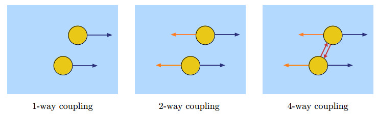
Furthermore, referring to Figure 2, we will group the models according to the degree of coupling between wind-flow and dispersed phase. The approach mainly depends on the volume fraction of the dispersed phase and three different situations can be distinguished ^[31,32]:

● 1-way coupling: The wind field is used to compute the dispersed phase field which is treated as a transported passive scalar without any feedback on the flow. 0$^{th}$-order and 1$^{st}$-order models usually have this basic level of coupling;

● 2-way coupling: The presence of the dispersed phase is taken into account in the computation of the wind flow. A 2-fluid formulation is always 2-way coupled because of the presence of coupling terms in the momentum equations;

● 4-way coupling: Particle-particle interactions are considered as well as the particulate feedbacks on the wind flow.

Regarding wind-blown particulate transport, as we have previously mentioned, different physical mechanisms are involved and need to be taken into account. Most of the situations deal with particulate material settled on the ground which can start moving thanks to momentum transfer from the wind-flow to the particles by means of the wall shear stress. As we shall see in the following section, this process generates both erosion and deposition zones, as well as initializes particulate material drift at the ground, large air entrainment and transport.

3.1.   Eulerian-Eulerian approach

Eulerian modeling of the dispersed phase was largely used for wind-blown snow, in order to predict erosion and deposition maps. From a mathematical point of view, whatever is the granular material considered, the modeling approach is the same. The advantage of an Eulerian-Eulerian approach mainly consists in the fact that it requires less computational resources compared to Lagrangian simulations, which were not even affordable years ago for industrial purposes.

Very early attempts of predicting particulate mass drift were done computing physical quantities along a constant wind direction. These models used two-dimensional domains and the variables are computed along a vertical plane. Recently, they have been also used to model dune migration, avoiding to compute the real sand transport in the air. Liston et al. ^[72] considered a quasi-steady two-dimensional case; only saltation is considered using the empirical expression in ^[91] to get snow saltation flux $Q_{sal}$ from the ground based on friction velocity (see Eq. (3.6) below). This idea was further developed in several other papers ^{[6,7,29,35,86,90,95,96,120]}. In this work we do not describe such models in further details, because they do not explicitly solve for the transport of particulate in the air.

The earliest attempt to obtain accurate deposition maps and snowdrift fields computing dispersed particle transport was done in the early nineties in ^[109]. In this model a diffusion equation for suspension transport is solved including a term accounting for the particle fall terminal velocity, while for the saltation flux a theoretical model based on friction velocity is employed. Wind flow fields are obtained by means of RANS approach with mixing-length turbulence closure. Erosion is computed using a heuristic expression for the saltation flux, while particle deposition is obtained assuming it to be proportional to the product of the density in the saltation layer and the settling velocity of particles. Erosion-deposition balance allows to compute the evolution of the ground surface. The model is then applied to both two-dimensional and three-dimensional cases with an assumed initial flat topography.

Gauer ^[36] has proposed a two-layer model applied to more complicated topographies. His idea consisted in dividing the domain in two zones: In one of them saltation is relevant, in the other one only suspension is considered. In the suspension layer an Eulerian-Eulerian approach with 1-way coupling is used. Wind flow fields are obtained by means of RANS $k$-$\epsilon$ model. In the saltation layer a 2-way coupling model is used, but the effect on turbulence due to the presence of particles is assumed negligible.

Similarly, Naaim et al. ^[82] presented an Eulerian-Eulerian $1^{st}$-order model with 1-way coupling based on mass conservation equations for fluid and dispersed phase separately, and a momentum equation for the mixture of air and particles, solved by RANS with a modified $k$-$\epsilon$ turbulence model, in order to considered the effect of the dispersed phase on turbulence. In particular, wind-blown particle transport is modeled distinguishing between saltation and suspension layer, yielding two different equations for particle concentrations, while a single momentum equation for the air-solid mixture.

In a slightly different way, a single transport equation is used in ^[3] and ^[2] adding a saltation source term at the first cell centers above the ground.

Bang et al. ^[11] and Sundsbø ^[103] paved the way to the use of Volume Of Fluid (VOF) for wind-blown particulate simulations, proposing a model of slip velocity between phases. Successively Beyers et al. ^[14,15] presented an Eulerian-Eulerian 1$^{st}$-order model with 1-way coupling, in which the balance equations of mass and momentum are solved for the mixture. Suspension and saltation are modeled separately. The former is described by a transport equation where the advection velocity is the sum of the velocity of the mixture and the slip velocity obtained using the drift flux model in ^[11].

More recently, Tominaga et al. ^[107] published a review of the CFD modeling of snowdrift around buildings. In the same work, they propose a model of wind-blown snow that solves suspension and saltation transport without distinguishing between them. It is an Eulerian-Eulerian $1^{st}$-order model with 1-way coupling, that treats the fluid-phase by means of the RANS $k$-$\epsilon$ model used in ^[82], but with optimized additional terms based on experiments. After few years a modification of the same $k$-$\epsilon$ model was proposed in ^[85].

Similarly to the above models, Eulerian-Eulerian models for wind-blown sand were used in ^[52] and ^[92] using 1-way coupling approaches, taking into account saltation by means of suitable viscosity coefficents.

The first Eulerian-Eulerian $2^{nd}$-order model with 2-way coupling was presented in ^[19]. Another novelty of this work is that two particle size distributions are simultaneously taken into account, leading to a significant improvement with respect to wind tunnel validation tests. Furthermore, Zhou et al. ^[119] presented a methodology that used the model in ^[107]. Based on meteorological data, the duration $T$ of certain snow drifts is divided into $n$ time windows. A steady solution is computed for each time-interval and the domain is modified and remeshed according to the resulting particulate drift.

3.1.1.   Modeling wind interaction with the ground and particle interaction with the wind

Eulerian approaches require suitable models describing interaction phenomena with the ground, that is, erosion, saltation-suspension transport, and deposit, as well as the effect of particles on turbulence. The models dealing with such phenomena will be described in the following subsections.

As already mentioned, continuum approaches have been largely used for snow drift-prediction. Therefore, most of the Eulerian dispersed particle models refers to snow. For this reason, part of the next subsections is done following the wind-blown-snow review ^[107], complementing it with the latest development and models related to different particulate materials.

Saltation and suspension transport modeling

Mathematical models developed for mass transport of sand and snow always consider saltation, because it is responsible of most of the particulate transport. Conversely, suspension has been usually considered negligible, or has been treated separately. Just few models have a single equation for both transport modes.

In particular, Eulerian dispersed particle transport was mainly modeled using one-fluid approaches, because particle velocity is not explicitly evaluated. The passive scalar transport equation models suspension transport, while saltation is often considered aside in a separated layer, or using empirical expressions at the first cell centers above the ground.

One of the earliest models was presented in ^[109] where the drift density $\Phi_s$ $[{kg}/{m^3}]$ was used as a transported scalar and it was assumed that the velocity of the dispersed phase is equal to that of the wind plus the particle-fall settling velocity. The transport equation then reads as:

where $u_w$ is the fall velocity considered constant and equal to the terminal settling velocity, while the turbulent diffusion term is modeled by means of Boussinesq's approximation

This approach was chosen in ^{[81,94,107,119]}, even though in the last two articles saltation is included in the transport equation originally written for suspension transport.

In a slightly different way Gauer ^[36] and Naaim et al. ^[82] distinguished between saltation and suspension layers applying respectively two different transport equations there.

The former used a 2-way coupling in the saltation layer, while no particle feedback on the flow is considered in the suspension layer. The latter considered a transport equation inside the saltation layer which takes into account of particle-mass exchange between saltation and suspension layers. They also considered a term present in the transport equation for the suspension layer as well with the opposite sign, in addition to particle-mass exchange between flow and ground surface. The equation for the suspension layer then reads as:

while that in the saltation layer is

where ${\bf q}_{ex}$ is the exchange between layers (obtained by the balance between diffusive and settling flux), ${\bf q}_{ground}$ is the flow-ground exchange term, which is equal to the erosion-deposition flux, whose expression will be detailed in the next section, $\Sigma_{sal}$ is the interface between saltation and suspension layer, and $\Sigma_{ground}$ is the interface between ground and saltation layer.

Other authors (e.g., ^{[14,15,94,109]}) evaluated the saltation flux $Q_{sal}$ at the first cell center above the ground, using empirical formulas based on the existence of a treshold shear velocity $u_{*, t}$ above which there is a saltation flux, or solving a balance equation. Different empirical formulations for the saltation flux $Q_{sal}$ in a saturated saltation layer in equilibrium conditions have been proposed. Defining $(f)_+ = (f+|f|)/2$ the positive part of $f$, the most used are the following:

● ^[49]:

where $C$ is an empirical constant

● ^[91]:

The former was for instance used in ^[109], the latter in ^[15,72,81] was sometimes used to evaluate an inlet particles-drift profile^[14].

Gauer ^[36] modelled saltation with a $2^{nd}$-order model with mass and momentum equations solved for the dispersed phase, using a scale analysis to simplify the expressions.

In the VOF and mixture theory framework, a transport equation similar to (3.3) has been proposed. The variable used is the dispersed volume fraction $\phi_s$, and the velocity used to advect it is the mixture velocity ${\bf U}$ plus the relative velocity ${\bf U}_r$:

where the turbulent diffusion term is modeled again with Boussinesq's approximation and in ^[11] the relative velocity is:

where $d$ is the mean diameter of the particles, approximated as spheres, $\hat\rho_s$ is the density of the particles of the dispersed phase. This transport equation was also used in ^[14,15,106].

Instead, in ^[2,3] Eq. (3.7) was adapted for the Fractional Area-Volume Obstacles Representation (FAVOR) method, which defines obstacles within a fluid computational domain, like VOF. Moreover, they added the following source term $S_{sal}$ accounting for saltation:

where $\beta_{sal} \in [0.15, 0.6]$.

The model presented in ^[103] also started from Eq. (3.7) (without diffusion term) to model saltation, while for suspension the drift velocity is assumed to be inversely proportional to air turbulence, in order to have that laminar regime gives the highest vertical fall velocity:

where $u_w = 0.3\ [m/s]$.

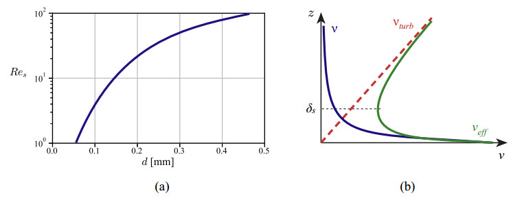
In the same spirt, Ji et al. ^[52] and Preziosi et al. ^[92] proposed a $1^{st}$-order model similar to (3.7), in which the convective velocity is the fluid velocity ${\bf u}$ plus a vertical component due to gravity. Moreover, saltation is included in the transport equation assuming a diffusive effect due to particles collision inside the saltation layer. This is done using an effective viscosity $\nu_{eff}$ inserted in the mass conservation equation:

While the model in ^[92] is a 1-way coupling, the one in ^[52] is a 2-way coupling model, due to the presence of momentum-extraction term in the fluid phase momentum balance equation.

In fact, on the basis of experimental data, the following form for the effective viscosity was proposed in ^[52]:

where $\beta = 0.217$ and

is the length scale of the saltation layer thickness and

where $d_1 = 2.5\cdot10^{-4}\; [m]$ and $d$ is the particle diameter ^[83].

Regarding the sedimentation velocity $u_w$, it can be classically calculated by the balance of drag and buoyancy forces and it strongly depends on the grain size (see, for instance, ^[38] or ^[34]). For small particle Reynolds numbers:

Stokes law gives:

Snow flakes certainly satisfy this regime. In case of particle Reynolds numbers in the range $[100, 1000]$ the sedimentation velocity is usually given in terms of the drag coefficient $C_D$

where $C_D$ can be approximated according to several experimental fittings (see, for instance, ^{[8,9,12,13,28,33,34,38,88,105,112]}).

In particular, in ^[52] has been used the relation

also suggested in ^[97].

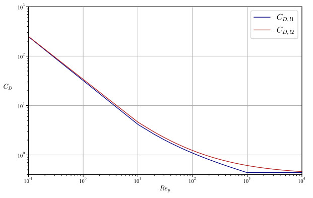
In ^[92] it was observed that it is useful to plot the experimental relationship between particle Reynolds number and drag in terms of a relationship between the grain size and the particle Reynolds number, as shown in Figure 3. For sand close to the ground the particle Reynolds number is typically between 1 and 100, while, as already stated, for snow flakes it is well below 1. Hence, while for snow it is possible to use Stokes law (3.13) for sand it is hard to find an explicit relationship and one has to rely on the experimental curves, such as those given in ^[12].

A further observation in ^[92] regards the effective viscosity $\nu_{eff}$ defined as the sum of molecular viscosity, turbulent viscosity and a term related to collisions inside the saltation layer. Regarding this last term, it is observed that the behavior of the sand particles is isotropic. Hence, objectivity implies that $\nu_{coll}$ is a scalar isotropic function of the rate of strain tensor ${\bf D} = \frac{1}{2}(\nabla{\bf u}+\nabla{\bf u}^T)$. By the representation theorem of isotropic function, $\nu_{coll}$ can then only depend on the invariants of ${\bf D}$ in addition to the density of the dispersed particles. However, since the flow can be considered as a perturbation of a shear flow in the vertical plane, the leading contribution is the second invariant $II_{\bf D} = \frac{1}{2}[({\rm tr}{\bf D})^2 - {\rm tr}({\bf D}^2)]$. For this reason, one can assume that $\nu_{coll} = \nu_{coll}(II_{\bf D}, \phi_s)$.

Boutanios and Jasak ^[19] proposed a $2^{nd}$-order model (2-fluid formulation) with a 2-way coupling, where there is no need to approximate the dispersed phase-velocity. The conservation of mass and momentum for both phases reads:

where $k = 0, 1$ respectively for the fluid and the dispersed phase, ${\bf g} = -g{{\bf e}_z}$ is the acceleration of gravity, ${\bf m}$ is the momentum exchange term (with opposite sign in the two equations), ${\bf T}_f$ is modelled as a viscous stress tensor. Considering that the equations are written for two-dimensional cases corresponding to a vertical plane, the viscosity $\nu_s$ is obtained starting from momentum balance for two-dimensional fully-developed steady-state flow containing dispersed-phase bed particles in a control volume, getting

where $\epsilon_s$ is the rate of strain of the dispersed phase, $x$ is the along-wind direction and $\tau_t = \hat\rho_s\phi_s u_*^2$ is the threshold shear stress.

Bed-surface evolution, erosion/deposit modeling

Bed-surface changes due to erosion and deposition of granular material should be accurately reproduced in order to get a reliable morphodynamic evolution and mass-drift results. This aspect is relevant both for its influence on the aerodynamics and for the information it carries on the accumulation zones.

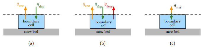
Referring to Figure 4, all models are based on a balance $q_{net}$ between deposition $q_{dep}$ and erosion $q_{ero}$ fluxes, that is written either as $q_{net} = q_{dep}+q_{ero}$ or as:

Considering a cell laying on the bed surface, the height change in a time interval $\Delta t$ is

where $A_{bed}$ is the area of the ground-face of the cell considered. If $q_{net} > 0$ deposition occurs, otherwise the sand-bed is eroded.

Several relationships have been suggested. For instance, referring to Figure 4(a), Uematsu et al. ^[109] proposed:

where $u_{sal}$ and $h_{sal}$ are respectively wind velocity in the saltation layer and saltation layer height.

Referring to Figure 4(c), Naaim et al. ^[82] suggested:

where $u_{*, r} = u_*-(u_*-u_{*, t})\frac{\Phi_s^2}{\Phi_{s, max}^2}$ and $\Phi_{s, max} = 0.248$ [kg/m]$^3$ for snow, recently used also in ^[102].

Referring to Figure 4(b), Beyers snd Sundsbø ^[14] computed fluxes differently and included a term taking into account of the impinging flow on the bed, so that the net flux is

with

where $C$ is a constant which represents the solid material pack bonding strength, $K$ is another model constant, $u_p$ is the flow velocity on the ground boundary cells, $n$ is related to granular surface features, $f(\alpha)$ is a function of the flow incident angle $\alpha$.

Referring to Figure 5, Beyers and Waechter ^[15] considered the mass balance equation

where

with $\beta = \frac{u_w}{\kappa u_*}$ and it is stated that

where ${\bf t}$ is the direction of the flow.

The quantities $q_{dep}$ and $q_{ero}$ are given by

where $u_{f, z}$ is the vertical component of fluid velocity and $u_{wt} = 0.4\sqrt{\frac{2}{3}k}$ is turbulent diffusion velocity, given by the isotropic turbulent velocity fluctuation approximation of the $k$-$\epsilon$ model, and

All the quantities are computed at the centers of the cells lying on the ground interface.

Tominaga et al. ^[107] proposed to model erosion on a flat bed as a turbulent-diffusion process:

This formula is used as a boundary condition for $\Phi_s$ ($z$ is the vertical direction normal to the flat plane), computing $q_{ero}$ by means of the empirical formula suggested in ^[4] for snow:

On the other hand, $q_{dep}$ is modeled as in ^[109] (see Eq. (3.19)).

A similar formula for the erosion flux was used in ^[92] on the basis of recent experiments reported in ^[41,42,43], who proposed

where $w_{ej} = 0.5\; m/s$ is the sand grain ejection velocity evaluated experimentally in ^{[26,41,42,43]}, $\alpha$ is a dimensionless free parameter to be fitted to experimental sand flux profiles, and

where $A_H$ is a model parameter depending of the physical properties of the granular material.

Erosion and deposition fluxes are almost always used in unsteady simulations to move the ground boundary or for domain re-meshing in order to have a boundary-fitted computational grid. Mesh-updating can take place at every time-step (as done in ^[14,15,107]), or when significant changes arise (as done in ^[36,82]), because wind flow and particles-deposit evolve with different time scales. Another way used to take this difference into account is a quasi-steady procedure, that consists in computing a steady solution for the wind phase, which is then used to evaluate mass drift and modify the domain. This procedure is then repeated. In this framework, one of the most recent developments is a multi-time step domain decomposition method for transport problems proposed in ^[21].

Less recent studies adopted instead a fill-cell technique that consists in computing the amount of volume occupied by the dispersed phase in the ground boundary cells and to exclude them from the domain when they are filled ^[2,3,72].

Particle effect on turbulence

In the suspension layer the concentration of particles is very low and the effect on turbulence is neglected in most of the articles. Naaim et al. ^[82] were the first to consider the influence of the dispersed phase on turbulence in a 1-way coupled model. They used a modified $k$-$\epsilon$ model ^[23] where the source terms

are respectively added to Eqs. (2.11) and (2.12) in order to take into account of the dissipative effect of the diluted phase. In Eqs. (3.32) and (3.33) $t^* = \frac{d^2\hat\rho_s}{18 \mu_f}$ is the dispersed particle relaxation time.

Tominaga et al. ^[107] used the same equations, but the additional terms were modified to:

where $C_{ks}$, $C_{\epsilon s}$ are constants, and $f_s$ is an exponential damping function.

Okaze et al. ^[85] proposed a new $k$-$\epsilon$ modified model for particles dispersed in the wind. Particles are thought as moving obstacles and modeled using vehicle canopy theory, i.e., canopy model concept for moving obstacles (see ^[79]).

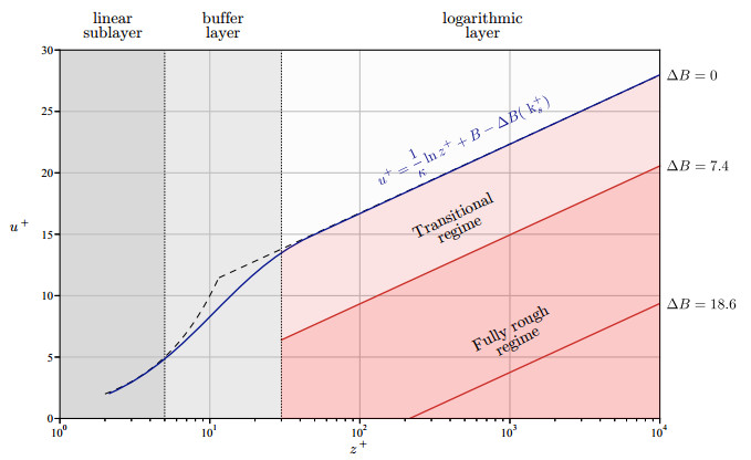
Considering that the concentration of particles is higher in the saltation layer, the following modification (based on measured data) of standard rough wall functions is proposed in ^[14] (see also ^[18]):

where:

● $B = 5.5$ is an integration constant,

● $\Delta B(k^+_s, s^+) = \frac{1}{\kappa} \text{ln}(1+0.3k^+_s+9, 53s^+)$ represents the intercept of the profile, switched from the origin due to roughness height,

● $k^+_s = \dfrac{k_su_*}{\nu_f}$ is the so-called dimensionless physical roughness height or roughness Reynolds number,

● $s^+ = \dfrac{c_1u^{3}_* }{2g\nu_f}$ is the additional parameter which models the effect of saltating particles, where $c_1$ is an empirical constant.

Defining:

● $z^+ = \dfrac{z_0 u_*}{\nu_f}$ the dimensionless wall distance,

● $u^+ = \dfrac{u }{u_*}$ the dimensionless velocity,

Eq. (3.36) can be written as $u^+ = \frac{1}{k}\ln(z^+)+B -\Delta B(k^+_s, s^+)$. Figure 6 shows the standard law proposed in ^[18] for different roughness regimes.

3.1.2.   Granular Kinetic Theory

A different Eulerian approach, called Granular Kinetic Theory (GKT) in analogy with the Gas Kinetic Theory ^[22], was proposed for dispersed particles multiphase simulations. The main idea of GKT consists in adopting a statistical and probabilistic approach to describe particle-particle interactions including both collision and friction, and random particles paths. In light of this approach, many quantities are introduced to describe sand dynamics. The most important one is the granular temperature that measures the energy level of the particle velocity fluctuations, which are then related to the air field by means of a turbulence model (generally a $k$-$\epsilon$ model). The solid pressure, that has the same meaning as pressure in gas standard models, describes the spherical component of the stress tensor for the dispersed phase. In this way, GKT models couple dispersed phase with carrying fluid behavior.

Specifically, Jenkins and Hanes ^[51] implemented a simple GKT model for a one-dimensional steady sheet flow focusing on a highly concentrated region of grains close to a sand bed, obtaining a qualitative good estimate of the erosion. The previous work was extended in ^[87] by implementing an extra term in the fluid momentum equation, following a modification suggested in ^[45]. They described an additional mechanism of suspension due to turbulence and granular pressure gradient. However, the results overestimated sand mass flux in comparison with experiments.

A further extension was proposed by Marval et al.^[76] who considered slightly anelastic particle-particle collisions and incorporated an improved two-dimensional transient model with a frictional sub-model to describe the sustained contacts between particles. The simulation results provided a good estimate of mass flux in sediment transport layer.

To our knowledge, at present the latest extension of the model consists in a 2$^{nd}$-order model with 2-way coupling ^[74]. This type of models involves many equations and thermodynamic parameters, hence here we show the main equations only. Working under the saturation assumption $\phi_f + \phi_s = 1$, the mass and momentum balance equations for phases are:

As mass and momentum conservation equation are present for both phases, then this model can be classified as a second order model. In the above equations

is the solid stress tensor,

are the fluid stress tensors and

is the lift force. In addition, in (3.39) the pressure of the suspension phase is written as

where

and $\mu_s = \mu_{kin} + \mu_{coll} + \mu_{fric}$. Formulas of these three viscosity terms are omitted for sake of brevity.

Lun et al. ^[75] derived all the involved expressions considering the anelastic nature of particle collision (instantaneous-binary collisions). Lugo et al. ^[74] claim that the most important idea of this model consists in introducing, as mentioned earlier, a quantity called granular or solid temperature $\Theta$, which is a measure of the energy level due to the particle velocity fluctuation. In particular, splitting the solid velocity into a sum of mean and fluctuation components, i.e., ${{\bf u}_s = \langle{\bf u}_s\rangle+{\bf u}_s'}$, the definition of $\Theta$ is $\Theta: = \frac{1}{3}\langle ||{\bf u}_s'||^2 \rangle$. Similarly to the classical gas theory, solving the equation

it is possible to obtain the pressure for solid phase through the constitutive relationship (3.46).

Finally, the chosen equations for turbulence model are

with

and

For sake of brevity, we omit the others 13 equations of the model, that involve many thermodynamics parameters that have to be chosen to characterize the sand type and the flow regime. However, for reader's use the "List of Main Symbols" is provided at the beginning of this article.

Many two-dimensional simulations were conducted with good qualitative results. In particular, the solid-like characteristics of the sand bed and the air free flow outside the saltation zone were correctly reproduced, also from the quantitative point of view. On the other hand, at the large-scale erosion was overpredicted by 20% and at the small-scale the parameters of the model used in ^[44] (conductivity, solid viscosity, granular temperature and mean free path) strongly affect sediment transport layer thickness, which appears thinner than experimental measurements. As observed in ^[74] GKT models can provide a relatively good description of the saltation layer, but they require further studies on the coupling turbulence models and on the effect that the parameters have on the solution.

3.2.   Eulerian treatment of wind driven rain

A somewhat different approach needs to be used for wind-blown rain, because the dispersed phase is liquid and is not entrained in the airflow from the ground apart from extreme situations of little practical interest, e.g., in presence of very strong winds. Moreover, the main transport process is due to convection and sedimentation. To the best of our knowledge, Eulerian-Eulerian approach for wind driven rain (WDR) have been introduced pretty recently by Huang and Li ^[47,48]. They proposed a 2-fluid formulation for WDR with a 2-way coupling.

The air-phase is modeled with a 1-fluid approach (see Eqs. (2.4) and (2.5)) using both RANS with realisable $k$-$\epsilon$ ^[47] and LES ^[48] coupled with an SGS model proposed in ^[46].

The rain-phase is considered as a poly-dispersed fluid with $k$ components, one per raindrop size class. Both mass and momentum conservation equations are solved:

where $\hat\rho_\ell$ is the water density, $\phi_k$ and ${ {\bf u}}_k$ are respectively the volume fraction and the velocity of the $k$ size range class. At variance with snow and sand-drift models, the authors above do not model turbulent diffusion, justifying it by the discrete nature of rain.

The motion of rain is obtained by the combined effect of gravity (the first term on the r.h.s. of Eq. (3.54)) and wind drag (the second term on the r.h.s. of Eq. (3.54)), that is taken to be given by Stokes law:

The sum of these last terms over all $k$ size-range class is inserted with the opposite sign in the momentum equation for the air-phase for coupling.

In ^[66] a similar model is proposed, but there is no effect in the air momentum equations due to the interactions with the rain drops. The 1-way coupling approximation is justified by the fact that the volume ratio is smaller than $10^{-4}$. The model is then extended in ^[68], where the effect of turbulent dispersion is included by means of Boussinesq eddy viscosity approximation for the Reynolds stresses modeling. This model has been successfully used for civil engineering application, involving different building set-ups and was validated with experimental measurements ^[65,67,69]. A similar model was also used in ^[89]. Finally, Wang et al. ^[111] added the resulting drag term to the wind momentum equation so that the model can be classified as a 2-way coupling model.

However, Huang and Li ^[47,48] mentioned that other approaches (mainly Lagrangian and heuristics) can be selected for computational reasons. In fact, their model requires using very fine grids in order to reduce numerical diffusion, as well as solving partial differential equations for each class of raindrop size of the poly-disperse flow.

3.3.   Eulerian-Lagrangian approach

While for wind-blown snow Eulerian-Eulerian approaches are always preferred, for sand Eulerian-Lagrangian approaches have been widely used, both for the persistent granular nature of sand and for the existence of previous studies on granular matter in general.

Eulerian-Lagrangian models allow to focus on phenomena related to the behavior of single grains and to get information at the grain scale that cannot be obtained by fully Eulerian models and that are hard to be obtained experimentally. On the other hand, in order to be statistically representative for the real ensemble of sand grains, a sufficiently large set of particles needs to be introduced in the domain, which makes the method computationally expensive. Basically, the method consists in solving the equations of motion for each particle including collision dynamics, to get individual trajectories. For these reasons, in general these methods are preferred to study local-scale phenomena.

After an earlier attempt by Anderson and Haff ^[4] and later by Lakehal et al. ^[70], only in the last two decades such computational approaches have taken hold in the particular fields of application of interest in this review. In fact, starting with ^[101], different discrete particles models have been proposed, specifically named as Discrete Particle Methods (DPM) and Discrete Element Method (DEM).

Before describing the models in some details, we give an overview of their main features. Kang and coauthors ^{[56,57,58,59]} proposed a DPM for the granular phase joined with RANS two-phase equations for the transporting phase (see Eqs. (2.6) and (2.7)), because of the lower computational cost of Reynolds-averaged approach. A 2-way coupling is employed. Particle distribution, velocity and drag force were analyzed and compared with wind-tunnel data ^[56,57,58]. The effect of Magnus and Saffman forces have been included and studied in ^[59]. A $k$-$\epsilon$ turbulence model was generally used, except in ^[56], where a simpler one equation mixing length model was preferred.

Concerning the particle tracking model, translational and rotational equations of motion are solved, taking into account the torque due to shear stress (except in ^[57]), and applying a soft-sphere model for inter-particles collisions. The simulation set-up used in ^[56] differs from the others because the domain bottom boundary coincides with the ground, while in the others the fluid-solid interface is inside the domain.

More sophisticated models were also proposed in order to improve the reliability of computational simulations. For instance, concerning the fluid phase, RANS approaches were sometimes replaced by LES or Lattice-Boltzmann methods. Specifically:

● Tong and Huang ^[108] combined a DEM with 2-way coupling with LES (with dynamic SGS closure) to obtain a more realistic flow field;

● Li et al. ^[71] put more details and effort in the computation of the particle trajectories using a DEM with 4-way coupling combined with LES fluid simulation using Smagorinsky sub-grid model;

● Shi et al. ^[98] combined a 2-way Lagrangian tracking method with a Lattice-Boltzman approach for fluid flow.

● Jiang et al. ^[53] used LES with Lagrangian tracking to investigate the effect on turbulent flow structures, sand transport, and sand particle reverse motion over two-dimensional transverse dunes.

● Okaze et al. ^[84] used LES with coherent structure Smagorinsky model ^[61,62], coupled with a snow transport model, based on the interaction between turbulent flow structures and snow particle dispersion.

Concerning the dispersed phase, different improvements were tried:

● Xiao et al. ^[117] extended the model presented in ^[57] where mono-sized sand was used, including different particle size distributions, both Gaussian and uniform.

● Lopes et al. ^[73] tackled the presence of different time scales by means of a quasi-steady procedure based on a RANS $k$-$\epsilon$ model with 1-way coupling.

Most of the works using Lagrangian methods studied local saltation phenomena over a flat bed. Instead, Jiang and coauthors ^[53,54] used particle tracking over a sand dune in a two-dimensional configuration, and investigated the effect of the presence of grains on the air-flow.

The same kind of models has been used for rain droplets, with some simplifications. The first models to evaluate the impact of wind driven rain on buildings was presented in ^[24,25]. These models used a 1-way coupling and were based on steady air-flow simulation using RANS $k$-$\epsilon$ models. Lift forces were always neglected, as well as rebound, splash, run-off and resuspension. Similar models were proposed by Hangan ^[40] and Abadie and Mendes ^[1], who used both $k$-$\epsilon$ and $k$-$\omega$ RANS, according to the position inside the computational domain.

Finally, it is worth pointing out that Lagrangian models seem to treat all transport modes implicitly. Actually, this is true only if particle-particle and particle-bed interaction are taken into account. For instance, saltation is the result of complicate inter-particle collisions.

3.3.1.   Particle equations of motion

As already mentioned, almost all Eulerian-Lagrangian models refer to Discrete Particle Methods (DPM) and Discrete Element Method (DEM). These methods solve the equations of motion for each particle:

where $m_p$ is the mass of the particle, ${\bf u}_p$ its velocity, and ${\bf F}_p$ the resulting force acting on the particle, that includes drag and gravity. In some cases the rotational degrees of freedom are considered as well, so that also the equations of angular momentum are solved:

where $I_p$ is the momentum of inertia of the particle (that is assumed spherical) and ${\bf \Omega}_p$ its angular velocity.

Almost all Lagrangian models are 2-way coupled (except for ^[73]), because the effect of the presence of particles is included into the air-phase mass and momentum balance equations (Eqs. (2.6) and (2.7)), which depend on the air-phase volume fraction $\phi_f = 1-\sum_{i = 1}^{N_{d}} \phi_{s, i}$, where, considering poly-disperse flows, $\phi_{s, i}$ is the volume fraction of the $i$-dispersed phase, and $N_d$ is the number of dispersed phases. Moreover, in Eq. (2.7) there is the solid-fluid coupling term ${\bf f}_{drag}$ which is the resultant of the drag forces exerted by particles ^[117]:

where $\Delta v$ is the volume of the considered computational cell, $N$ is the total number of particles inside the cell and ${\bf F}_p^{dr}$ is the drag force acting on the $p$-particle, computed by means of empirical relations, for instance:

where $C_D$ is the drag coefficient ^[28]. As already stated after Eq. (3.15), several laws have been proposed for $C_D$ to fit experimental data. In ^{[57,71,73,101]} the following relations generalizing Eq. (3.14) to high particle Reynolds numbers is used:

Instead, in ^{[56,58,108,117]} the following expression was used:

to express the drag coefficient laws (3.60) and (3.61) are compared in Figure 7, and they notably differs only for high $Re_p$. As observed above for sand particles close to the ground $1\leq Re_p\leq 100$.

Also the models proposed in ^[54,98,108] belong to the 2-way coupling category, because they included the effect of particles on the fluid.

In order to get 4-way coupling models like in ^[71] particle-particle and particle-bed interactions ${\bf F}^{coll}$ to ${\bf F}_p$ need be considered. In this case, the resulting force on particle $p$ generally reads:

where ${\bf F}^{coll}_p$ can be modelled with different levels of accuracy.

DEM approaches are able to treat multi-contact interactions using mechanical elements (springs, dampers, etc...) to describe forces by means of hard-sphere and soft-sphere models, as well described in ^[27]. For instance, Kang and Guo ^[57] and Li et al. ^[71] split ${\bf F}^{coll}_p$ as

where ${\bf f}^c_{pq}$ is a contact force and ${\bf f}^d_{pq}$ a viscous damping force which vanish when the particle $q$ does not collide with the particle $p$. The expressions of the normal and tangential components of the contact and damping forces are:

● Normal contact force: $f^c_{pq, n} = -\dfrac{4}{3}E^*\sqrt{r^*\delta_n^3},$

● Tangential contact force: $f^c_{pq, t} = -\dfrac{\mu_s |f^c_{pq}|}{|\delta_t|} \left[ 1- \left(1-\dfrac{\text{min} \{|\delta_t|, \delta_{t, max} \} }{\delta_{t, max}} \right)^{3/2} \right] \delta_t\, ,$

● Normal viscous damping force: $f^d_{pq, n} = -\eta\left(6m_{pq}E^*\sqrt{r^*\delta_n}\right)^{1/2}v_{pq, n}\, ,$

● Tangential viscous damping force: $f^d_{pq, t} = -\eta \left(6m_{pq}\mu_s |f^c_{pq}| \dfrac{\sqrt{1- |\delta_t|/\delta_{t, max}} }{\delta_{t, max} }\right)^{1/2}v_{pq, t}\, ,$

where $\frac{1}{m_{pq}} = \frac{1}{m_p}+\frac{1}{m_q}$ and $\frac{1}{r^*} = \frac{1}{r_p}+\frac{1}{r_q}$ with $r_p$ and $r_q$ the radii of the particles $p$ and $q$. In the same way,

where $E_p$, $E_q$ and $\nu_p$, $\nu_q$ are respectively the Young modulus and the Poisson ratio of the particles $p$ and $q$. In addition, $\mu_s$ is the friction coefficient, $\eta$ is the damping coefficient, $\delta = (\delta_{t}, \delta_{n})$ is the displacement vector between the particles $p$ and $q$ splitted in tangential and normal components and, similarly, $v_{pq} = (v_{pq, t}, v_{pq, n})$ is the relative velocity between the consider couple of particles, again splitted into tangential and normal components.

In ^[56,58,59] the inter-particles interaction forces are given by:

where the summation terms are computed using a linear spring-damper model. In particular, the components of the interaction force are:

● Normal component

● Tangential component

where $k_s$ is the stiffness coefficient and the other coefficients are as above. In addition, rotational degrees of freedom are also considered, adding the equations

where ${\bf T}_{pq}$ is the torque due to collision forces, ${\bf T}_f = 8\pi r^3\mu_f \Big{(} \frac{1}{2} \nabla \times {\bf u}_f-{\bf \Omega}_p\Big{)}$ is the torque on a spherical particle due to the fluid shear stress. In ^[57,71] Eq. (3.65) is solved neglecting ${\bf T}_f$.

An alternative way to model particle-particle and particle-bed interactions consists in using a hard-sphere model with impulsive interaction forces. With this approach, particles restore their shape after impact. However, in this approach only instantaneous binary collisions are considered. Multiple interactions are neglected and so it can be used for dilute suspensions only and not close to the sand-bed. Considering two particles $p$ and $q$, conservation of linear and angular momentum reads:

where the index $(0)$ refers to the values of velocity and angular velocity before the collision and $\mathbf{J}$ is the impulsive force.

Such an approach was used by Sun et al. ^[101] who considered binary elastic collisions between non-deformable spheres, using analytical average normal and tangential impulses to compute velocity variations. In ^[117] hard-spheres were used to model both particle-particle and particle-bed interactions.

As far as rain droplets are concerned, most of the models are based on Choi's work ^[24,25]. In his model only translation motion is considered and in Eq. (3.56) the resulting force on a particle is a balance between Stokes drag and buoyancy:

Instead Hangan ^[40] used the following expression:

for the drag force in the rain droplet translation equation of motion, where $C_D = a_1+\frac{a_2}{Re}+\frac{a_3}{Re^2}$ is the drag coefficient given by Morsi-Alexander law. A similar quadratic dependence on the relative velocity was used in ^[1].

3.3.2.   Particles-bed interaction

The Lagrangian approach allows to avoid dynamical re-meshing, because the integration cell can be fixed and even be crossed by the ground surface. However, this implies to accurately model the interaction of the dispersed particles in the saltation and creep layer with those particles laying on the ground. One simple way to do that is to compose the ground surface using a set of motionless particles and a restitution coefficient. Two different initial particles-bed configurations, with 3000 and 5000 particles were studied in ^[57]. The former reaches a steady state in 3.6 seconds, while the latter in 3.4 seconds, even if a direct comparison between the two set-ups can not be made because the simulations differ in other parameters. Similarly, 8000 particles were used in ^[58].

Differently, in ^[56] the ground interface is outside the domain, under its bottom boundary. Therefore, no boundary model is applied, and the dynamics is totally simulated by means of inter-particles collision models.

On the contrary, Xiao et al. ^[117] focused on the effect of two different bed models:

● Flat bed model: The bed is considered as a motionless particle having an infinite mass (also used in ^[71]);

● Rough bed model: The bed is considered as a set of particles having mass and size of a settling particle; The velocity vector relative to an impacting particle and the wall is taken to be a Gaussian distribution.

The choice of bed models affects the results, and each of them seems to represent a particular type of sand surface (rough bed model) or desert areas (Gobi area, flat bed model).

Tong and Huang ^[108] and Jiang ^[53] modelled the impacting-ejecting process on the basis of the splash function proposed in ^[110,113]. Specifically, the rebound and the ejected speeds $v_{re}$ and $v_{ej}$, and the rebound and ejected angles $\alpha_{re}$ and $\alpha_{ej}$ are given by uniform probability densities with mean $|\bar v_{re}| = 0.3 |v_{im}|$ and $\bar \alpha_{re} = 0.60$, where $v_{im}$ is the impinging speed and $\alpha_{im}$ is the impinging angle. However, the reported values of the standard deviation deserve more studies because they are sometimes unphysical.

The number of ejected sand particles $N_p^{ej}$ is:

On the other hand, Shi et al. ^[98] chose the following Gamma distribution function

for the lift-off speed $v_0$ in order to capture the stochastic nature of the ejection process (see also ^[5]), while the number of particles ejected by splashing $N_p^{ej}$ and the rebound velocity and probability are following ^[113]

3.3.3.   Different time-scale treatment

Air and particles have very different characteristic time-scales. From a computational point of view, this aspect is cumbersome and needs to be carefully considered in order to avoid waste of computational resources. In Lagrangian simulations the multi-time-scale issue is tackled using different time steps to integrate the equations for particles and air, as reported in Table 1. In all cases there is one order of magnitude difference between particle and air time-step.

4.   Final Comments

In this work a wide overview of mathematical models for wind-blown particulate transport based on Computational Fluid Dynamics approach has been provided. Analyzing separately fully-Eulerian and Eulerian-Lagrangian models, the mathematical treatment of each physical process involved in particulate mass transport is described. In order to help making a comparison, the large set of models proposed in the literature for different dispersed multiphase flows has been presented and organized trying to homogenize the used mathematical frameworks.

A good comparison with experimental data in different contexts can be achieved by both discrete and continuous models. So, the choice of one model over another mainly depends on the application of interest. For instance, Eulerian-Lagrangian models can directly reproduce some dispersed particle behavior, but the large number of elements needed to get reliable statistical properties limits the size of the domains that can be investigated and eventually the range of applicability to engineering applications.

On the other hand, fully Eulerian approaches are much faster, but are based on continuum approximation or closures. Moreover, they require a bigger modeling effort, especially when a two-fluid formulation is adopted. An example of this difficulty is given by GKT models, that can reach good results, at the price of solving for many volume-averaged variables.

It seems then that continuum approaches are suitable for medium-large transport scales, while discrete ones are precious tools for studying locally some particular transport phenomena, such as saltation, creep, or splash and rebounding. In this respect, it is worth underlining that the results of one approach can be used to improve the lacks of the other. In particular, outputs from Lagrangian-Eulerian models can be used to identify some quantities characterizing fully Eulerian models.

Acknowledgments

This work was developed in the framework of the Wind-blown Sand Modeling and Mitigation joint research, development and consulting group established between Politecnico di Torino and Optiflow Company. It was partially funded by the Istituto Nazionale di Alta Matematica, Regione Piemonte and the European Union's Horizon 2020 research and innovation programme MSCA-ITN-2016-EID through the research project SMaRT (grant agreement No.721798).

Conflict of interest

The authors declare no conflict of interest.