This study aims to analyze lesions on computed tomography (CT) images and digital subtraction angiography (DSA) of ruptured cerebral arteriovenous malformation (AVM).
Cross-sectional description of 82 patients' cerebral bleeding due to rupture of AVM, determined by multislice computed tomography or cerebral DSA at Bach Mai Hospital.
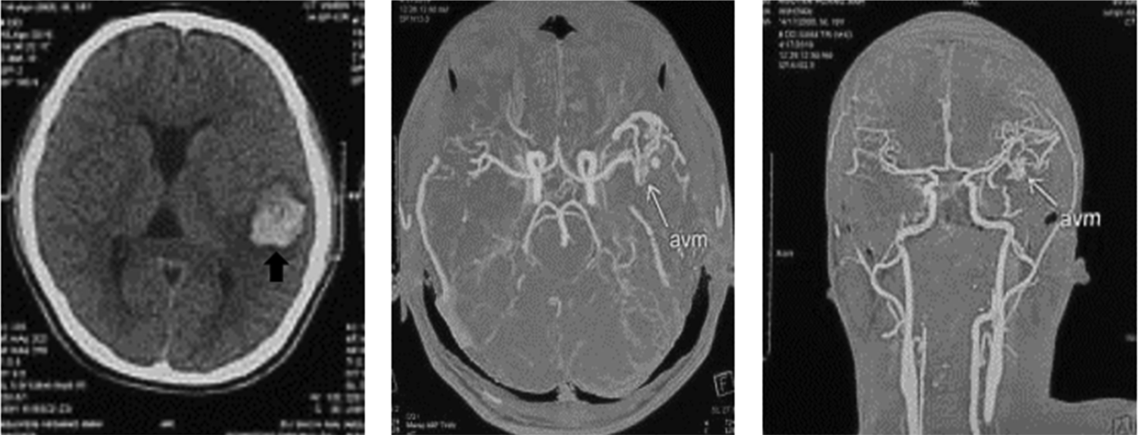
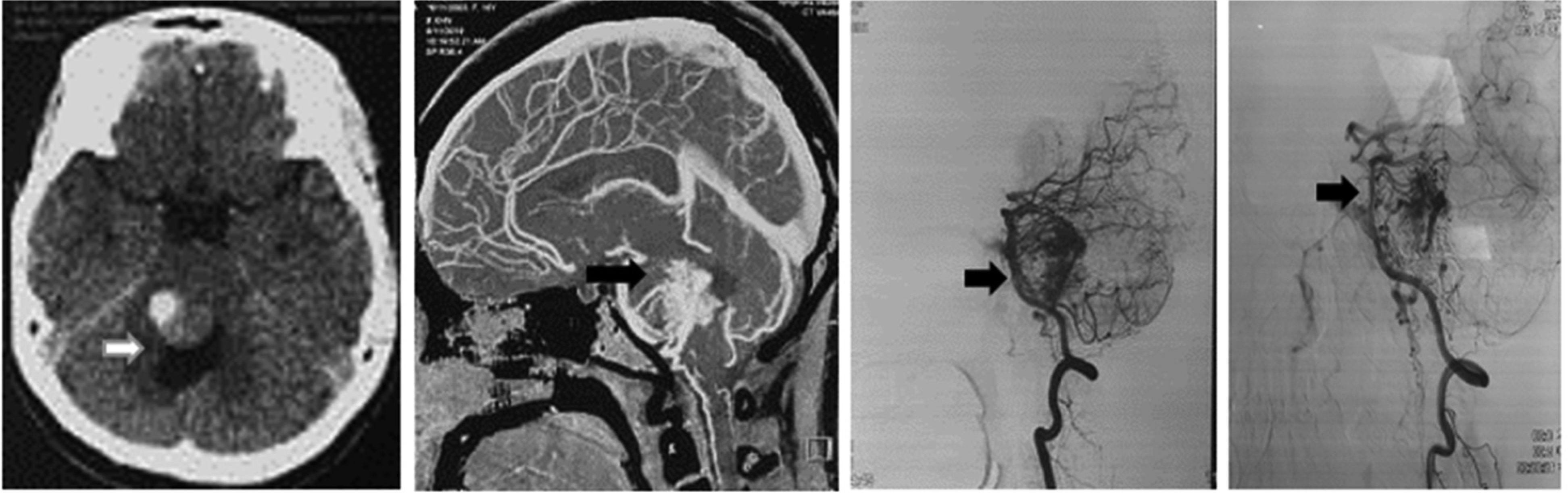
Patients with ruptured AVM are commonly under 40 years old (62.2%), average age: 35.1 ± 11.2. On CT or DSA images, it is common to see AVM rupture causing cerebral bleeding in the supratentorial region (91.5%), with 83% cerebral lobe bleeding, mainly small and moderate hematoma volume (<60 cm3) (74.4%), and a low rate of consciousness disorders (p < 0.05). AVM is usually found in the supratentorial region (91.5%), and the size is small (74.4%) (p < 0.05). The feeding arteries are mainly derived from the middle (53.7%) and posterior (42.7%) cerebral arteries; 70.7% is drained by superficial veins. According to the Spetzler–Martin classification, degrees I and II account for the highest percentage (73.2%), in which the majority of patients are selected for surgery; grades IV and V have a low rate (8.5%), often a combination of vascular and surgical nodes.
On MSCT and DSA images, ruptured AVMs often cause lobar hemorrhage in young people. AVMs are usually small to moderate in size. The feeding arteries are mainly derived from middle and posterior cerebral arteries, and drained mainly by superficial veins. The Spetzler–Martin classification and the supplementary grading scales are used for ranking the severity of the lesion, as well as for choosing AVM treatment options and assessing the prognosis.
Citation: Van Tuan Nguyen, Anh Tuan Tran, Nguyen Quyen Le, Thi Huong Nguyen. The features of computed tomography and digital subtraction angiography images of ruptured cerebral arteriovenous malformation[J]. AIMS Medical Science, 2021, 8(2): 105-115. doi: 10.3934/medsci.2021011
This study aims to analyze lesions on computed tomography (CT) images and digital subtraction angiography (DSA) of ruptured cerebral arteriovenous malformation (AVM).
Cross-sectional description of 82 patients' cerebral bleeding due to rupture of AVM, determined by multislice computed tomography or cerebral DSA at Bach Mai Hospital.
Patients with ruptured AVM are commonly under 40 years old (62.2%), average age: 35.1 ± 11.2. On CT or DSA images, it is common to see AVM rupture causing cerebral bleeding in the supratentorial region (91.5%), with 83% cerebral lobe bleeding, mainly small and moderate hematoma volume (<60 cm3) (74.4%), and a low rate of consciousness disorders (p < 0.05). AVM is usually found in the supratentorial region (91.5%), and the size is small (74.4%) (p < 0.05). The feeding arteries are mainly derived from the middle (53.7%) and posterior (42.7%) cerebral arteries; 70.7% is drained by superficial veins. According to the Spetzler–Martin classification, degrees I and II account for the highest percentage (73.2%), in which the majority of patients are selected for surgery; grades IV and V have a low rate (8.5%), often a combination of vascular and surgical nodes.
On MSCT and DSA images, ruptured AVMs often cause lobar hemorrhage in young people. AVMs are usually small to moderate in size. The feeding arteries are mainly derived from middle and posterior cerebral arteries, and drained mainly by superficial veins. The Spetzler–Martin classification and the supplementary grading scales are used for ranking the severity of the lesion, as well as for choosing AVM treatment options and assessing the prognosis.

| [1] | Bokhari MR, Bokhari SRA (2020) Arteriovenous Malformation of the Brain Treasure Island (FL): StatPearls Publishing. |
| [2] |
Tranvinh E, Heit JJ, Hacein-Bey L, et al. (2017) Contemporary imaging of cerebral arteriovenous malformations. AJR Am J Roentgenol 208: 1320-1330. doi: 10.2214/AJR.16.17306

|
| [3] | Li TL, Fang B, He XY, et al. (2005) Complication analysis of 469 brain arteriovenous malformations treated with N-butyl cyanoacrylate. Interv Neuroradiol 11: 141-148. |
| [4] |
Ujiie H, Tamano Y, Xiuling L, et al. (2000) Haemorrhagic complication after total extirpation of huge arteriovenous malformations. J Clin Neurosci 7: 73-77. doi: 10.1016/S0967-5868(00)90716-1
|
| [5] |
Rutledge WC, Ko NU, Lawton MT, et al. (2014) Hemorrhage rates and risk factors in the natural history course of brain arteriovenous malformations. Transl Stroke Res 5: 538-542. doi: 10.1007/s12975-014-0351-0
|
| [6] |
Wang H, Ye X, Gao X, et al. (2014) The diagnosis of arteriovenous malformations by 4D-CTA: a clinical study. J Neuroradiol 41: 117-123. doi: 10.1016/j.neurad.2013.04.004
|
| [7] |
Anderson JL, Khattab MH, Sherry AD, et al. (2020) Improved cerebral arteriovenous malformation obliteration with 3-Dimensional rotational digital subtraction angiography for radiosurgical planning: a retrospective cohort study. Neurosurgery 88: 122-130. doi: 10.1093/neuros/nyaa321
|
| [8] |
Conti A, Friso F, Tomasello F (2020) Commentary: improved cerebral arteriovenous malformation obliteration with 3-Dimensional rotational digital subtraction angiography for radiosurgical planning: a retrospective cohort study. Neurosurgery 88: E33-E34. doi: 10.1093/neuros/nyaa409
|
| [9] |
Hakim A, Mosimann PJ (2020) Intracranial arteriovenous malformation: cinematic rendering with digital subtraction angiography. Radiology 294: 506. doi: 10.1148/radiol.2019192083
|
| [10] |
Spetzler RF, Martin NA (1986) A proposed grading system for arteriovenous malformations. J Neurosurg 65: 476-483. doi: 10.3171/jns.1986.65.4.0476
|
| [11] |
Lawton MT, Kim H, McCulloch CE, et al. (2010) A supplementary grading scale for selecting patients with brain arteriovenous malformations for surgery. Neurosurgery 66: 702-713. doi: 10.1227/01.NEU.0000367555.16733.E1
|
| [12] |
Duong DH, Young WL, Vang MC, et al. (1998) Feeding artery pressure and venous drainage pattern are primary determinants of hemorrhage from cerebral arteriovenous malformations. Stroke 29: 1167-1176. doi: 10.1161/01.STR.29.6.1167
|
| [13] |
Murthy SB, Merkler AE, Omran SS, et al. (2017) Outcomes after intracerebral hemorrhage from arteriovenous malformations. Neurology 88: 1882-1888. doi: 10.1212/WNL.0000000000003935
|
| [14] |
Stefani MA, Porter PJ, terBrugge KG, et al. (2002) Large and deep brain arteriovenous malformations are associated with risk of future hemorrhage. Stroke 33: 1220-1224. doi: 10.1161/01.STR.0000013738.53113.33
|
| [15] |
van Rooij WJ, Jacobs S, Sluzewski M, et al. (2012) Endovascular treatment of ruptured brain AVMs in the acute phase of hemorrhage. AJNR Am J Neuroradiol 33: 1162-1166. doi: 10.3174/ajnr.A2995
|
| [16] |
Iosif C, Mendes GA, Saleme S, et al. (2015) Endovascular transvenous cure for ruptured brain arteriovenous malformations in complex cases with high Spetzler-Martin grades. J Neurosurg 122: 1229-1238. doi: 10.3171/2014.9.JNS141714
|
| [17] | Steiger HJ, Schmid-Elsaesser R, Muacevic A, et al. (2002) Neurosurgery of Arteriovenous Malformations and Fistulas: A multimodal approach Springer-Verlag Vienna. |
Figures(2) / Tables(7)

Van Tuan Nguyen, Anh Tuan Tran, Nguyen Quyen Le, Thi Huong Nguyen. The features of computed tomography and digital subtraction angiography images of ruptured cerebral arteriovenous malformation[J]. AIMS Medical Science, 2021, 8(2): 105-115. doi: 10.3934/medsci.2021011


 DownLoad: