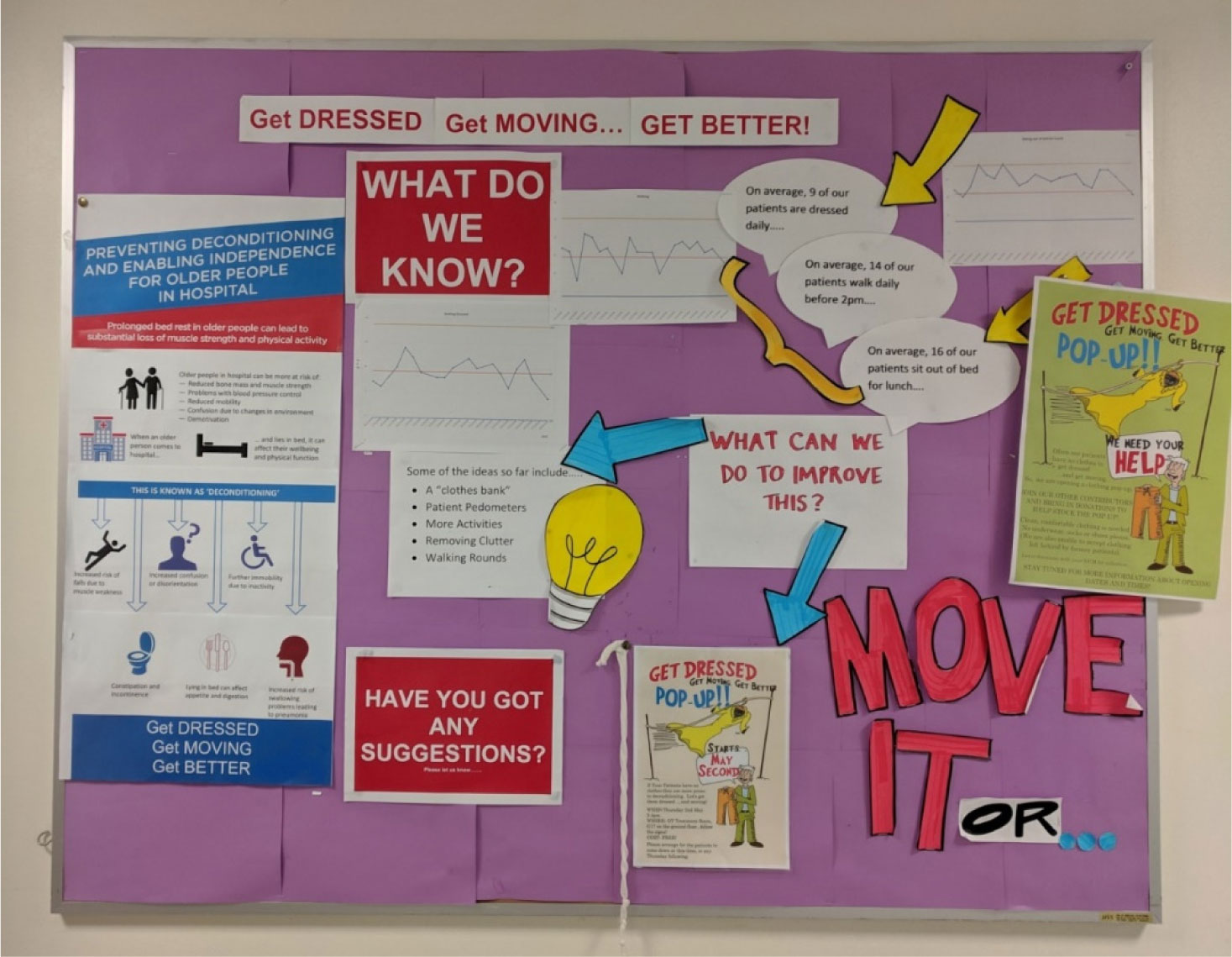
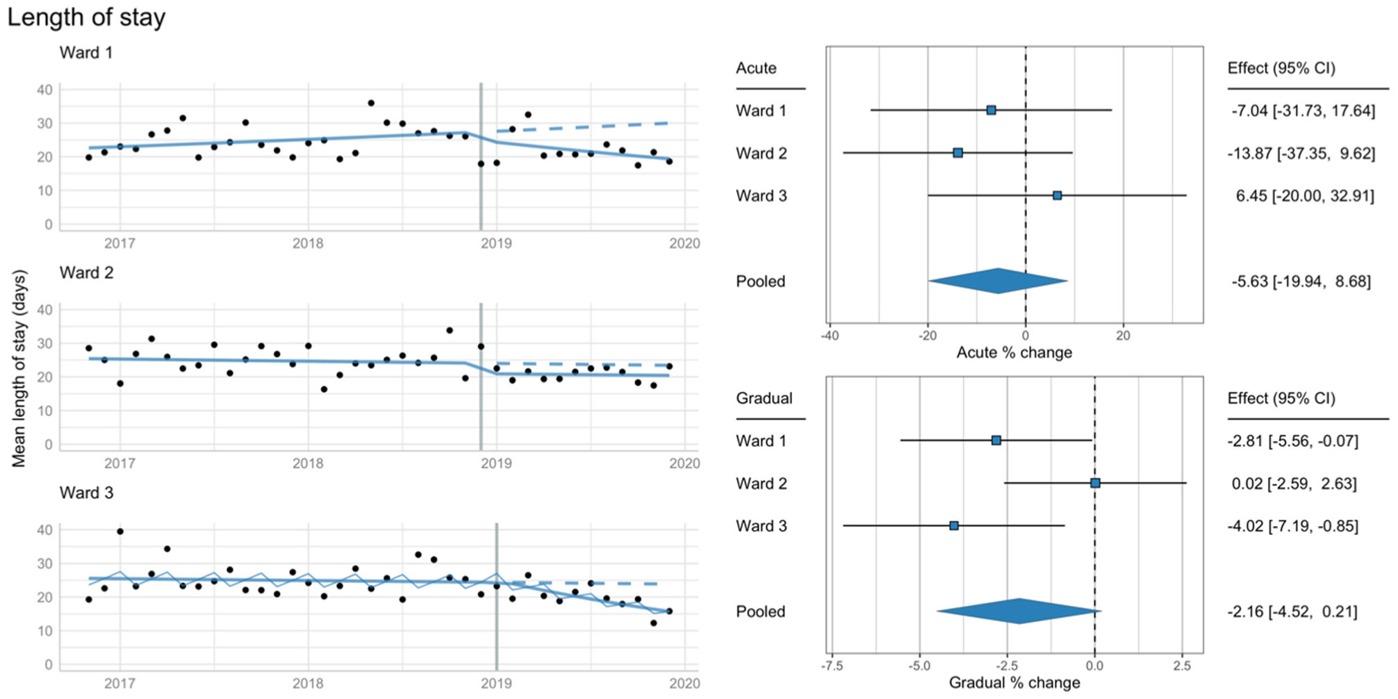
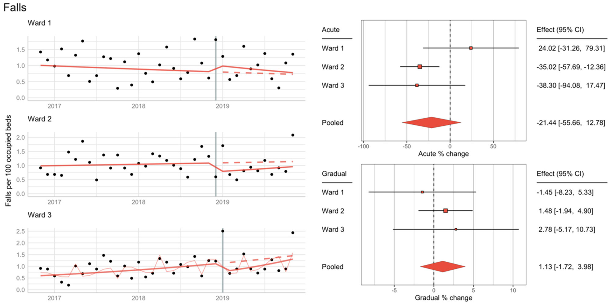
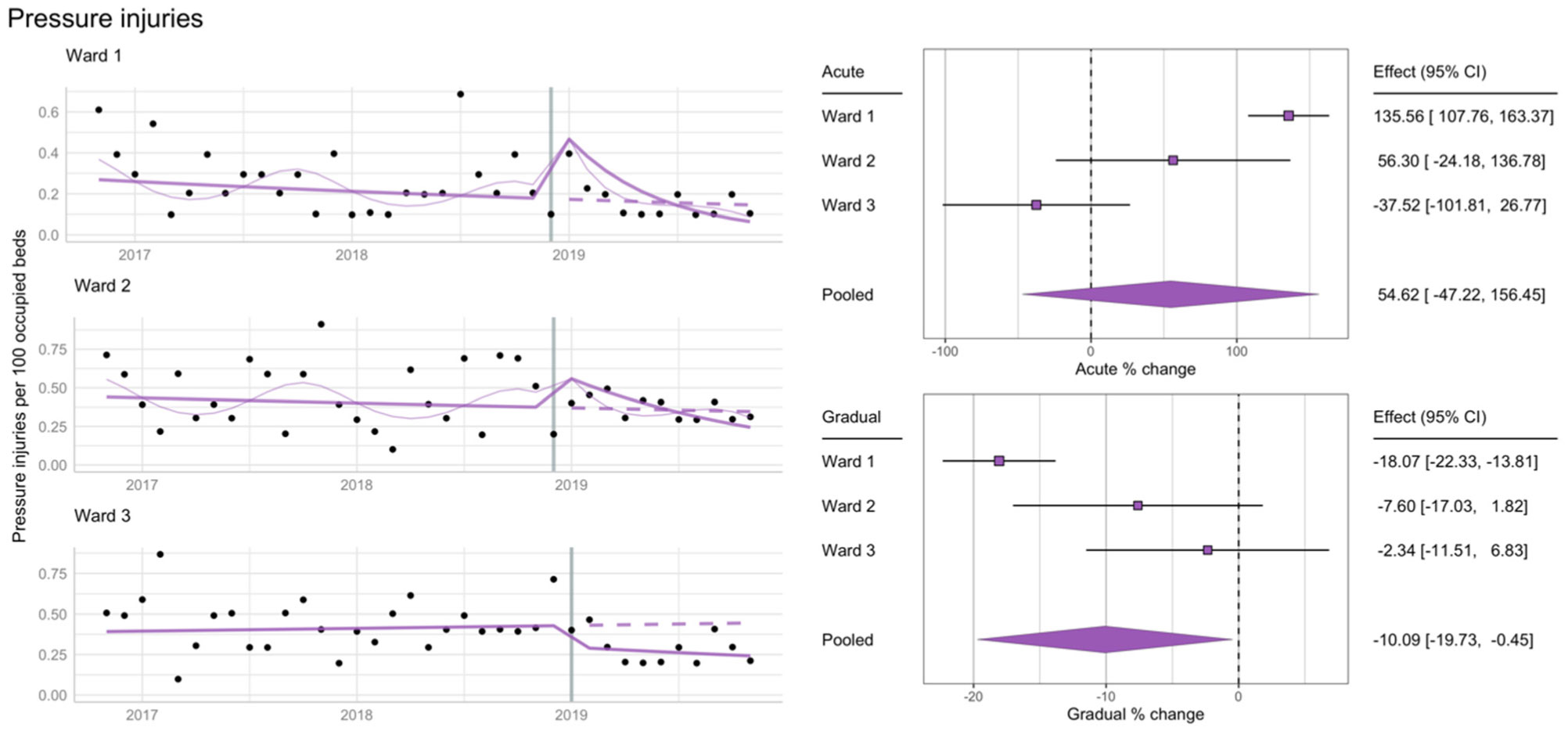
The “End-PJ-Paralysis” social movement has promoted global recognition of the problem of low activity levels for hospitalised older adults, but whether aligned quality improvement programmes impact length of stay or adverse events is unknown. To determine the impact of a multicomponent intervention, which included data displays, exercise groups, a clothing repository, widespread promotion, and targeted education for staff and patients to promote dressing and activity, we conducted an interrupted time series analysis. Although there was no clear impact upon length of stay or fall or pressure rates after 12 months, this is an important finding for other centres implementing their own “End-PJ-Paralysis” interventions as it highlights that such programmes are not associated with increased falls, as commonly feared.
Citation: Amelia Crabtree, Tyler J Lane, Lisa Mahon, Taryn Petch, Christina L Ekegren. The impact of an End-PJ-Paralysis quality improvement intervention in post-acute care: an interrupted time series analysis[J]. AIMS Medical Science, 2021, 8(1): 23-35. doi: 10.3934/medsci.2021003
The “End-PJ-Paralysis” social movement has promoted global recognition of the problem of low activity levels for hospitalised older adults, but whether aligned quality improvement programmes impact length of stay or adverse events is unknown. To determine the impact of a multicomponent intervention, which included data displays, exercise groups, a clothing repository, widespread promotion, and targeted education for staff and patients to promote dressing and activity, we conducted an interrupted time series analysis. Although there was no clear impact upon length of stay or fall or pressure rates after 12 months, this is an important finding for other centres implementing their own “End-PJ-Paralysis” interventions as it highlights that such programmes are not associated with increased falls, as commonly feared.

| [1] |
Greysen S (2016) Activating hospitalized older patients to confront the epidemic of low mobility. JAMA Intern Med 176: 928-929. doi: 10.1001/jamainternmed.2016.1874

|
| [2] |
Growdon M, Shorr R, Inouye S (2017) The tension between promoting mobility and preventing falls in the hospital. JAMA Intern Med 177: 759-760. doi: 10.1001/jamainternmed.2017.0840
|
| [3] |
Brown C, Redden D, Flood K, et al. (2009) The underrecognized epidemic of low mobility during hospitalization of older adults. J Am Geriatr Soc 57: 1660-1665. doi: 10.1111/j.1532-5415.2009.02393.x
|
| [4] |
Grant P, Granat M, Thow M, et al. (2010) Analyzing free-living physical activity of older adults in different environments using body-worn activity monitors. J Aging Phys Act 18: 171-184. doi: 10.1123/japa.18.2.171
|
| [5] |
Kortebein P, Ferrando A, Lombeida J, et al. (2007) Effect of 10 days of bed rest on skeletal muscle in healthy older adults. JAMA 297: 1772-1774. doi: 10.1001/jama.297.16.1772-b
|
| [6] |
Kortebein P, Symons T, Ferrando A, et al. (2008) Functional impact of 10 days of bed rest in healthy older adults. J Gerontol A Biol Sci Med Sci 63: 1076-1081. doi: 10.1093/gerona/63.10.1076
|
| [7] |
Brown C, Friedkin R, Inouye S (2004) Prevalence and outcomes of low mobility in hospitalized older patients. J Am Geriatr Soc 52: 1263-1270. doi: 10.1111/j.1532-5415.2004.52354.x
|
| [8] |
Fisher S, Graham J, Ottenbacher K, et al. (2016) Inpatient walking activity to predict readmission in older adults. Arch Phys Med Rehabil 97: S226-231. doi: 10.1016/j.apmr.2015.09.029
|
| [9] |
Agmon M, Zisberg A, Gil E, et al. (2017) Association between 900 steps a day and functional decline in older hospitalized patients. JAMA Intern Med 177: 272-274. doi: 10.1001/jamainternmed.2016.7266
|
| [10] |
Pavon J, Sloane R, Pieper C, et al. (2020) Accelerometer-measured hospital physical activity and hospital-acquired disability in older adults. J Am Geriatr Soc 68: 261-265. doi: 10.1111/jgs.16231
|
| [11] |
Chastin S, Harvey J, Dall P, et al. (2019) Beyond “#endpjparalysis”, tackling sedentary behaviour in health care. AIMS Med Sci 6: 67-75. doi: 10.3934/medsci.2019.1.67
|
| [12] |
Mavroeidi A, McInally L, Tomasella F, et al. (2019) An explorative study of current strategies to reduce sedentary behaviour in hospital wards. AIMS Med Sci 6: 285-295. doi: 10.3934/medsci.2019.4.285
|
| [13] | Health Service 360 End PJ Paralysis (2020) .Available from: https://endpjparalysis.org/. |
| [14] |
Oliver D (2017) David Oliver: Fighting pyjama paralysis in hospital wards. BMJ 357: j2096. doi: 10.1136/bmj.j2096
|
| [15] |
Moreno N, de Aquino B, Garcia I, et al. (2019) Physiotherapist advice to older inpatients about the importance of staying physically active during hospitalisation reduces sedentary time, increases daily steps and preserves mobility: a randomised trial. J Physiother 65: 208-214. doi: 10.1016/j.jphys.2019.08.006
|
| [16] |
Hshieh T, Yang T, Gartaganis SL, et al. (2018) Hospital elder life program: systematic review and meta-analysis of effectiveness. Am J Geriatr Psychiatry 26: 1015-1033. doi: 10.1016/j.jagp.2018.06.007
|
| [17] |
Hastings S, Sloane R, Morey M, et al. (2014) Assisted early mobility for hospitalized older veterans: preliminary data from the STRIDE program. J Am Geriatr Soc 62: 2180-2184. doi: 10.1111/jgs.13095
|
| [18] |
Brown C, Foley K, Lowman J, et al. (2016) Comparison of posthospitalization function and community mobility in hospital mobility program and usual care patients: a randomized clinical trial. JAMA Intern Med 176: 921-927. doi: 10.1001/jamainternmed.2016.1870
|
| [19] |
Brown C, Williams B, Woodby L, et al. (2007) Barriers to mobility during hospitalization from the perspectives of older patients and their nurses and physicians. J Hosp Med 2: 305-313. doi: 10.1002/jhm.209
|
| [20] |
Inouye S, Brown C, Tinetti M (2009) Medicare nonpayment, hospital falls, and unintended consequences. N Engl J Med 360: 2390-2393. doi: 10.1056/NEJMp0900963
|
| [21] |
Smart D, Dermody G, Coronado M, et al. (2018) Mobility programs for the hospitalized older adult: a scoping review. Gerontol Geriatr Med 4: 2333721418808146. doi: 10.1177/2333721418808146
|
| [22] | Shadish W, Cook T, Campbell D (2002) Experimental and Quasi-Experimental Designs for Generalized Causal Inference Boston: Houghton Mifflin. |
| [23] |
Penfold R, Zhang F (2013) Use of interrupted time series analysis in evaluating health care quality improvements. Acad Pediatr 13: S38-S44. doi: 10.1016/j.acap.2013.08.002
|
| [24] | Get Dressed, Get Moving, Get BETTER! [video file] 2019 Available from: https://www.youtube.com/watch?v=w6_yEnbOyhk. |
| [25] | Cowpertwait P, Metcalfe A (2009) Introductory Time Series with R New York: Springer. |
| [26] |
Jebb A, Tay L (2017) Introduction to time series analysis for organizational research. Organ Res Methods 20: 61-94. doi: 10.1177/1094428116668035
|
| [27] | Fox J, Weisberg S (2018) Time-series regression and generalized least squares: an appendix to an r companion to applied regression. An R Companion to Applied Regression Los Angeles: Sage, 1-8. |
| [28] |
Viechtbauer W (2010) Conducting meta-analyses in R with the metafor package. J Stat Softw 36: 1-48. doi: 10.18637/jss.v036.i03
|
| [29] | Lane T, Crabtree A, Mahon L, et al. (2020) Analytical code: the impact of a multicomponent End-PJ-Paralysis quality improvement intervention in post-acute care: an interrupted time series analysis. Bridges Available from: <https://bridges.monash.edu/articles/code/Analytical_code_The_impact_of_a_multicomponent_End-PJ-Paralysis_quality_improvement_intervention_in_post-acute_care_an_interrupted_time_series_analysis_/12798119>. |
| [30] |
McCullagh R, Dillon C, Dahly D, et al. (2016) Walking in hospital is associated with a shorter length of stay in older medical inpatients. Physiol Meas 37: 1872-1884. doi: 10.1088/0967-3334/37/10/1872
|
| [31] |
Azuh O, Gammon H, Burmeister C, et al. (2016) Benefits of early active mobility in the medical intensive care unit: a pilot study. Am J Med 129: 866-871. E1. doi: 10.1016/j.amjmed.2016.03.032
|
 medsci-08-01-003-s001.pdf medsci-08-01-003-s001.pdf |
 |
Figures(5)

Amelia Crabtree, Tyler J Lane, Lisa Mahon, Taryn Petch, Christina L Ekegren. The impact of an End-PJ-Paralysis quality improvement intervention in post-acute care: an interrupted time series analysis[J]. AIMS Medical Science, 2021, 8(1): 23-35. doi: 10.3934/medsci.2021003


 DownLoad: