Cerebral Connectivity and High-grade Gliomas: Evolving Concepts of Eloquent Brain in Surgery for Glioma

Sanjay Konakondla; Steven A. Toms; Sanjay Konakondla; Steven A. Toms

doi:10.3934/medsci.2017.1.52

AIMS Medical Science

2017, Volume 4, Issue 1: 52-70. doi: 10.3934/medsci.2017.1.52

Previous Article Next Article

Review

Cerebral Connectivity and High-grade Gliomas: Evolving Concepts of Eloquent Brain in Surgery for Glioma

Sanjay Konakondla ^{1
,
,},
Steven A. Toms ²

1.
Geisinger Health System, 100 N. Academy Drive, Danville, PA 17822, USA;
2.
Rhode Island Hospital, 593 Eddy Street, Providence, RI 02903, USA

Received: 22 November 2016 Accepted: 22 January 2017 Published: 05 February 2017

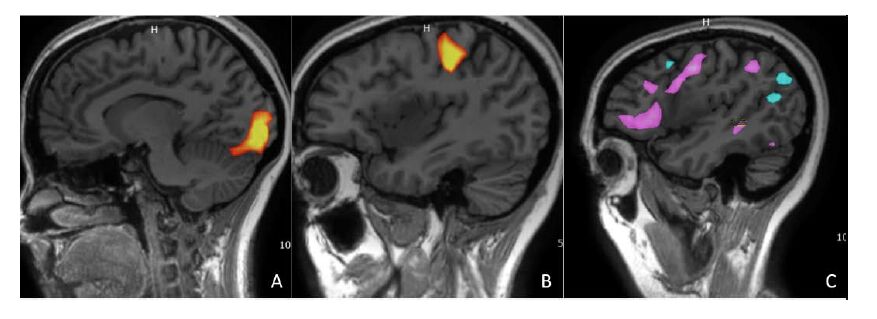
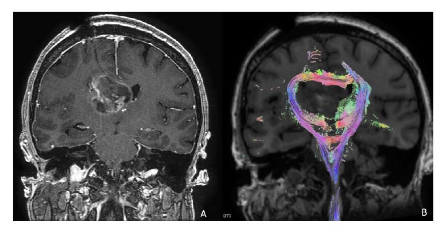
Technological advances in imaging the human brain help us map and understand the intricacies of cerebral connectivity. Current techniques and specific imaging sequences, however, do come with limitations. Image resolution, variability of techniques and interpretation of images across institutions are just a few concerns. In the setting of high-grade gliomas, understanding how these pathways are affected during tumor growth, surgical resection, and in the brain plasticity presents an even greater challenge. Clinical symptoms, tumor growth, and intraoperative electrical stimulation are important peri-operative considerations to assist in determining neuronal re-wiring and establish a basis of anatomic and functional correlation. The application of functional mapping coupled with the understanding of the natural history of gliomas and implications of neural plasticity, is critical in achieving the goals of maximal tumor resection while minimizing post operative deficits and improving quality of life.

Keywords:

Citation: Sanjay Konakondla, Steven A. Toms. Cerebral Connectivity and High-grade Gliomas: Evolving Concepts of Eloquent Brain in Surgery for Glioma[J]. AIMS Medical Science, 2017, 4(1): 52-70. doi: 10.3934/medsci.2017.1.52

Related Papers:

[1]	M. Mossa Al-Sawalha, Rasool Shah, Adnan Khan, Osama Y. Ababneh, Thongchai Botmart . Fractional view analysis of Kersten-Krasil'shchik coupled KdV-mKdV systems with non-singular kernel derivatives. AIMS Mathematics, 2022, 7(10): 18334-18359. doi: 10.3934/math.20221010
[2]	M. Mossa Al-Sawalha, Osama Y. Ababneh, Rasool Shah, Amjad khan, Kamsing Nonlaopon . Numerical analysis of fractional-order Whitham-Broer-Kaup equations with non-singular kernel operators. AIMS Mathematics, 2023, 8(1): 2308-2336. doi: 10.3934/math.2023120
[3]	Reetika Chawla, Komal Deswal, Devendra Kumar, Dumitru Baleanu . A novel finite difference based numerical approach for Modified Atangana- Baleanu Caputo derivative. AIMS Mathematics, 2022, 7(9): 17252-17268. doi: 10.3934/math.2022950
[4]	Naveed Iqbal, Saleh Alshammari, Thongchai Botmart . Evaluation of regularized long-wave equation via Caputo and Caputo-Fabrizio fractional derivatives. AIMS Mathematics, 2022, 7(11): 20401-20419. doi: 10.3934/math.20221118
[5]	Gulalai, Shabir Ahmad, Fathalla Ali Rihan, Aman Ullah, Qasem M. Al-Mdallal, Ali Akgül . Nonlinear analysis of a nonlinear modified KdV equation under Atangana Baleanu Caputo derivative. AIMS Mathematics, 2022, 7(5): 7847-7865. doi: 10.3934/math.2022439
[6]	Khalid Khan, Amir Ali, Manuel De la Sen, Muhammad Irfan . Localized modes in time-fractional modified coupled Korteweg-de Vries equation with singular and non-singular kernels. AIMS Mathematics, 2022, 7(2): 1580-1602. doi: 10.3934/math.2022092
[7]	Ahu Ercan . Comparative analysis for fractional nonlinear Sturm-Liouville equations with singular and non-singular kernels. AIMS Mathematics, 2022, 7(7): 13325-13343. doi: 10.3934/math.2022736
[8]	Saima Rashid, Rehana Ashraf, Fahd Jarad . Strong interaction of Jafari decomposition method with nonlinear fractional-order partial differential equations arising in plasma via the singular and nonsingular kernels. AIMS Mathematics, 2022, 7(5): 7936-7963. doi: 10.3934/math.2022444
[9]	Changdev P. Jadhav, Tanisha B. Dale, Vaijanath L. Chinchane, Asha B. Nale, Sabri T. M. Thabet, Imed Kedim, Miguel Vivas-Cortez . On solutions of fractional differential equations for the mechanical oscillations by using the Laplace transform. AIMS Mathematics, 2024, 9(11): 32629-32645. doi: 10.3934/math.20241562
[10]	Saima Rashid, Sobia Sultana, Bushra Kanwal, Fahd Jarad, Aasma Khalid . Fuzzy fractional estimates of Swift-Hohenberg model obtained using the Atangana-Baleanu fractional derivative operator. AIMS Mathematics, 2022, 7(9): 16067-16101. doi: 10.3934/math.2022880

Abstract

1. Introduction

In a letter to L'Hospital in 1695, the famous mathematician Leibniz introduced the concept of fractional derivative for the first time. Fractional calculus is concerned with non-integral differential and integral operators. The integer-order differential operator is a local operator, but the fractional-order differential operator is non-local, indicating that a system's next state is determined not only by its current state but also by all of its past states. It is more realistic, which is one of the main reasons for the popularity of fractional calculus. Fractional calculus was found to be more suitable for modelling real-world problems than classical calculus. The theory of fractional calculus provides an effective and systematic interpretation of nature's reality. The following are some basic works on fractional calculus on various topics, such as Podlubny ^[1], Caputo ^[2], Kiryakova ^[3], Jafari and Seifi ^[4,5], Momani and Shawagfeh ^[6], Oldham and Spanier ^[7], Diethelm et al. ^[8], Miller and Ross ^[9], Kemple and Beyer ^[10], Kilbas and Trujillo ^[11].

Fractional differential equations (FDEs) are widely widely used in various fields of science. FDEs have attracted a lot of attention in the last few years because of their diverse uses in physics and engineering. Due to its proven usefulness in a wide range of very diverse disciplines of science and engineering, fractional partial differential equations (PDEs) have gained importance and reputation among FDEs in recent years. For example, fractional derivatives in a fluid-dynamic traffic model can be utilised to overcome the insufficiency produced by the assumption of a continuous flow of traffic. Nonlinear FPDE solutions are of tremendous interest in both mathematics and practical applications ^{[12,13,14,15,16,17,18,19,20,21]}. The world's most important processes are represented by nonlinear equations. Manipulation of nonlinear processes is essential in physics, applied mathematics, and engineering problems. The significance of finding the exact solution to nonlinear partial differential equations is still a prominent issue in physics and applied mathematics, requiring implemented using different techniques to determine new approximate or exact solutions ^{[22,23,24,25]}.

In order to obtain explicit solutions for nonlinear equations of integer order, various techniques have been used. To solve FPDEs, however, only a less numerous approaches are used. such as Laplace variational iteration method (LVIM) ^[26], iterative Laplace transform method (ILTM) ^[27], optimal Homotopy asymptotic method (OHAM)^[28], approximate-analytical method (AAM) ^[29], reduced differential transform method (RDTM) ^[30], Laplace-Adomian decomposition method (LADM) ^[31], natural transform decomposition method (NTDM) ^[32], Elzaki transform decomposition method (ETDM) ^[33,34,35], new meshfree technique (NMT) ^{[36,37,38,39,40]}, Homotopy analysis method (HAM) ^[41], generalized exponential rational function method (GERFM) ^[42,43] and much more ^{[44,45,46,47,48,49,50,51]}. The goal of this paper is to implement the natural decomposition approach to solve modified Boussinesq equations and approximate long wave equations having fractional-order. Natural decomposition methods avoid roundoff errors by not requiring prescriptive assumptions, linearization, discretization, or perturbation.

Whitham ^[52], Broer ^[53], and Kaup ^[54] discovered the Whitham-Broer-Kaup (WBK) equations in the twentieth century, which describe the propagation of shallow water waves with various dispersion relations. Consider the fractional order coupled WBK equations ^[55]:

$\begin{equation} \begin{split} \frac{\partial^\wp{u}}{\partial{\Im^\wp}}&+u\frac{\partial u}{\partial {\xi}}+\frac{\partial v}{\partial {\xi}}+b\frac{\partial^{2} u}{\partial {\xi}^{2}} = 0, \\ \frac{\partial^\wp{v}}{\partial{\Im^\wp}}&+u\frac{\partial v}{\partial {\xi}}+v\frac{\partial u}{\partial {\xi}}+a\frac{\partial^{3} u}{\partial {\xi}^{3}}-b\frac{\partial^{2} v}{\partial {\xi}^{2}} = 0, 0 < \wp\leq 1. \end{split} \end{equation}$

(1.1)

where $v = v(\xi, \tau)$ is the height that deviates from the liquid's equilibrium position and $u = u(\xi, \tau)$ is the horizontal velocity. The order of the time-fractional derivative is in this case. Furthermore, a and b are constants that represent different diffusion strengths, therefore Eq (1.1) becomes a modified Boussinesq equation if $a = 1$ and $b = 0$ . Similarly, the system denotes the standard long wave equation for $a = 0$ and $b = 1.$ These equations are used in ocean and coastal engineering to explain the propagation of waves in dissipative and nonlinear media. They are recommended for situations involving water leakage in porous subsurface stratum and are frequently used in hydrodynamics. Furthermore, Eq (1.1) serves as the foundation for a number of models that represent the unconfined subsurface, such as drainage and groundwater problems ^[56,57].

The following is a summary of the paper's structure. The essential definitions related to fractional calculus are briefly discussed in Section 2. The NTDM is a method implemented to solve coupled WBK equations having fractional order with non-singular definitions are given in Section 3. In Section 4, we discussed the uniqueness and convergence results. Two examples of fractional-order modified Boussinesq and approximate long wave equations are given in Section 5 to validate the approaches. The article's brief conclusions are offered in Section 6.

2. Basic preliminaries

In the literature, there are various fractional derivative definitions; for additional details, see ^[58,59,60]. This section includes Caputo, Riemann-Liouville, Atangana-Baleanu and Caputo-Fabrizio definitions for the benefit of the readers.

Definition 2.1. For a function $h\in C_{v}, v\geq-1$ , the Riemann-Liouville fractional integral operator is given as ^[61]

$\begin{equation} \begin{split} I^{{{\wp}}}h(\eta) = &\frac{1}{\Gamma({{\wp}})}\int_{0}^{\eta}(\eta-\zeta)^{{{\wp}}-1}h(\zeta)d\zeta, \ \ {{\wp}} > 0, \ \ \eta > 0.\\ \ \ I^{0}h(\eta) = &h(\eta). \end{split} \end{equation}$

(2.1)

Definition 2.2. The fractional derivative $h(\eta)$ in Caputo manner is given as ^[61]

$\begin{equation} \begin{split} D_{\eta}^{{{\wp}}}h(\eta) = I^{{m}-{{\wp}}}D^{{m}}h(\eta) = \frac{1}{{m}-{{\wp}}}\int_{0}^{\eta}(\eta-\zeta)^{{m}-{{\wp}}-1}h^{{m}}(\zeta)d\zeta, \end{split} \end{equation}$

(2.2)

for ${m}-1 < {{\wp}}\leq {m}, \ \ {m}\in N, \ \ \eta > 0, h\in C^{{m}}_{v}, v\geq-1$ .

Definition 2.3. Caputo-Fabrizio fractional derivative for $h(\eta)$ is given as ^[61]

$\begin{equation} \begin{split} D_{\eta}^{{{\wp}}}h(\eta) = \frac{F({{\wp}})}{1-{{\wp}}}\int^{\eta}_{0}\exp\left(\frac{-{{\wp}}(\eta-\zeta)}{1-{{\wp}}}\right)D(h(\zeta))d\zeta, \end{split} \end{equation}$

(2.3)

where $0 < {{\wp}} < 1$ and $F({{\wp}})$ is a normalization function with $F(0) = F(1) = 1$ .

Definition 2.4. The Atangana-Baleanu Caputo derivative of fractional-order for $h(\eta)$ is defined as ^[61]

$\begin{equation} \begin{split} D_{\eta}^{{{\wp}}}h(\eta) = \frac{B({{\wp}})}{1-{{\wp}}}\int^{\eta}_{0}E_{{{\wp}}}\left(\frac{-{{\wp}}(\eta-\zeta)}{1-{{\wp}}}\right)D(h(\zeta))d\zeta, \end{split} \end{equation}$

(2.4)

where $0 < {{\wp}} < 1$ , where $B(\wp)$ is Normalization function and $E_{{{\wp}}}(z) = \sum_{m = 0}^{\infty}\frac{z^{m}}{\Gamma({{\wp}}^{m}+1)}$ is the Mittag-Leffler function.

Definition 2.5. For a function $u(\Im)$ , the Natural transformation is defined as

$\begin{equation} \begin{split} \mathcal{N}(u(\Im)) = \mathcal{U}({s}, {{\vartheta}}) = \int_{-\infty}^{\infty}e^{-s\Im}u(\vartheta\Im)d\Im, \ \ s, {\vartheta}\in (-\infty, \infty). \end{split} \end{equation}$

(2.5)

Natural transformation of $u(\Im)$ for $\Im\in(0, \infty)$ is given as

$\begin{equation} \begin{split} \mathcal{N}(u(\Im)H(\Im)) = \mathcal{N}^{+} = \mathcal{U}^{+}({s}, {{\vartheta}}) = \int_{-\infty}^{\infty}e^{-s\Im}u(\vartheta\Im)d\Im, \ \ s, {\vartheta}\in (0, \infty). \end{split} \end{equation}$

(2.6)

here $H(\Im)$ is the Heaviside function.

Definition 2.6. For a function $\mathcal{U}({s}, {{\vartheta}})$ , the Natural inverse transformation is given as

$\begin{equation} \begin{split} \mathcal{N}^{-1}[\mathcal{U}({s}, {{\vartheta}})] = u(\Im), \ \ \forall \Im\geq0. \end{split} \end{equation}$

(2.7)

Lemma 2.1. If linearity property having Natural transformation for $u_{1}(\Im)$ is $u_{1}({s}, {{\vartheta}})$ and $u_{2}(\Im)$ is $u_{2}({s}, {{\vartheta}})$ , then

$\begin{equation} \begin{split} \mathcal{N}[c_{1}u_{1}(\Im)+c_{2}u_{2}(\Im)] = c_{1}\mathcal{N}[u_{1}(\Im)]+c_{2}\mathcal{N}[u_{2}(\Im)] = c_{1}\mathcal{U}_{1}({s}, {{\vartheta}})+c_{2}\mathcal{U}_{2}({s}, {{\vartheta}}), \end{split} \end{equation}$

(2.8)

where $c_{1}$ and $c_{2}$ are constants.

Lemma 2.2. If Natural inverse transformation of $\mathcal{U}_{1}({s}, {{\vartheta}})$ and $\mathcal{U}_{2}({s}, {{\vartheta}})$ are $u_{1}(\Im)$ and $u_{2}(\Im)$ respectivelythen

$\begin{equation} \begin{split} \mathcal{N}^{-1}[c_{1}\mathcal{U}_{1}({s}, {{\vartheta}})+c_{2}\mathcal{U}_{2}({s}, {{\vartheta}})] = c_{1}\mathcal{N}^{-1}[\mathcal{U}_{1}({s}, {{\vartheta}})]+c_{2}\mathcal{N}^{-1}[\mathcal{U}_{2}({s}, {{\vartheta}})] = c_{1}u_{1}(\Im)+c_{2}u_{2}(\Im), \end{split} \end{equation}$

(2.9)

where $c_{1}$ and $c_{2}$ are constants.

Definition 2.7. The Natural transformation of Caputo operator $D_{\Im}^{{{\wp}}}u(\Im)$ is define as ^[61]

$\begin{equation} \begin{split} \mathcal{N}[D_{\Im}^{{{\wp}}}u(\Im)] = \left(\frac{s}{{\vartheta}}\right)^{{{\wp}}}\left(\mathcal{N}[u(\Im)]-\left(\frac{1}{s}\right)u(0)\right). \end{split} \end{equation}$

(2.10)

Definition 2.8. In terms of Caputo-Fabrizio, the Natural transformation of $D_{\Im}^{{{\wp}}}u(\Im)$ is given as ^[61]

$\begin{equation} \begin{split} \mathcal{N}[D_{\Im}^{{{\wp}}}u(\Im)] = \frac{1}{1-{{\wp}}+{{\wp}}(\frac{{\vartheta}}{s})}\left(\mathcal{N}[u(\Im)]-\left(\frac{1}{s}\right)u(0)\right). \end{split} \end{equation}$

(2.11)

Definition 2.9. In terms of Atangana-Baleanu Caputo derivative, the Natural transformation of $D_{\Im}^{{{\wp}}}u(\Im)$ is defined as ^[61]

$\begin{equation} \begin{split} \mathcal{N}[D_{\Im}^{{{\wp}}}u(\Im)] = \frac{M[{{\wp}}]}{1-{{\wp}}+{{\wp}}(\frac{{\vartheta}}{s})^{{{\wp}}}}\left(\mathcal{N}[u(\Im)]-\left(\frac{1}{s}\right)u(0)\right). \end{split} \end{equation}$

(2.12)

3. Methodology

This section introduces a general numerical methodology based on the Natural transform for the following equation.

$\begin{equation} \begin{split} D_{\Im}^{{{\wp}}}\nu(\xi, \Im) = \mathcal{L}(\nu(\xi, \Im))+\mathbb{N}(\nu(\xi, \Im))+h(\xi, \Im), \end{split} \end{equation}$

(3.1)

with initial source

$\begin{equation} \begin{split} \nu(\xi, 0) = \phi(\xi), \end{split} \end{equation}$

(3.2)

here $\mathcal{L}$ is linear, $\mathbb{N}$ is nonlinear and $h(\xi, \Im)$ represents source term.

3.1. Case Ⅰ $(NTDM_{CF}):$

We get this by applying Caputo-Fabrizio fractional derivative with the aid of Natural transformation of Eq (3.1),

$\begin{equation} \begin{split} \frac{1}{p({{\wp}}, {{\vartheta}}, {s})}\left(\mathcal{N}[\nu(\xi, \Im)]-\frac{\phi(\xi)}{s}\right) = \mathcal{N}[M(\xi, \Im)], \end{split} \end{equation}$

(3.3)

where

$\begin{equation} \begin{split} p({{\wp}}, {{\vartheta}}, {s}) = 1-{{\wp}}+{{\wp}}(\frac{{\vartheta}}{s}). \end{split} \end{equation}$

(3.4)

We may express Eq (3.3) as, using the inverse Natural transformation

$\begin{equation} \begin{split} \nu(\xi, \Im) = \mathcal{N}^{-1}\left(\frac{\phi(\xi)}{s}+p({{\wp}}, {{\vartheta}}, {s})\mathcal{N}[M(\xi, \Im)]\right), \end{split} \end{equation}$

(3.5)

$\mathbb{N}(\nu(\xi, \Im))$ can be decomposed into

$\begin{equation} \begin{split} \mathbb{N}(\nu(\xi, \Im)) = \sum\limits_{i = 0}^{\infty}A_{i}, \end{split} \end{equation}$

(3.6)

where the Adomian polynomials is represented by $A_{\Im}$ .We assume that the numerical solution of Eq (3.1) exists

$\begin{equation} \begin{split} \nu(\xi, \Im) = \sum\limits_{i = 0}^{\infty}\nu_{i}(\xi, \Im). \end{split} \end{equation}$

(3.7)

By putting Eqs (3.6) and (3.7) into (3.5), we get

$\begin{equation} \begin{split} \sum\limits_{i = 0}^{\infty}\nu_{i}(\xi, \Im) = &\mathcal{N}^{-1}\left(\frac{\phi(\xi)}{s}+p({{\wp}}, {{\vartheta}}, {s})\mathcal{N}[h(\xi, \Im)]\right)\\ &+\mathcal{N}^{-1}\left(p({{\wp}}, {{\vartheta}}, {s})\mathcal{N}\left[\sum\limits_{i = 0}^{\infty}\mathcal{L}(\nu_{i}(\xi, \Im))+A_{\Im}\right]\right). \end{split} \end{equation}$

(3.8)

From (3.8), we obtain

$\begin{equation} \begin{split} \nu_{0}^{CF}(\xi, \Im) = &\mathcal{N}^{-1}\left(\frac{\phi(\xi)}{s}+p({{\wp}}, {{\vartheta}}, {s})\mathcal{N}[h(\xi, \Im)]\right), \\ \nu_{1}^{CF}(\xi, \Im) = &\mathcal{N}^{-1}\left(p({{\wp}}, {{\vartheta}}, {s})\mathcal{N}\left[\mathcal{L}(\nu_{0}(\xi, \Im))+A_{0}\right]\right), \\ &\vdots\\ \nu_{l+1}^{CF}(\xi, \Im) = &\mathcal{N}^{-1}\left(p({{\wp}}, {{\vartheta}}, {s})\mathcal{N}\left[\mathcal{L}(\nu_{l}(\xi, \Im))+A_{l}\right]\right), \ \ l = 1, 2, 3, \cdots\\ \end{split} \end{equation}$

(3.9)

we obtain the $NTDM_{CF}$ solution of (3.1) by putting (3.9) into (3.7),

$\begin{equation} \begin{split} \nu^{CF}(\xi, \Im) = \nu_{0}^{CF}(\xi, \Im)+\nu_{1}^{CF}(\xi, \Im)+\nu_{2}^{CF}(\xi, \Im)+\cdots. \end{split} \end{equation}$

(3.10)

3.2. Case Ⅱ $(NTDM_{ABC}):$

We get this by applying Atangana-Baleanu derivative with the aid of Natural transformation of Eq (3.1),

$\begin{equation} \begin{split} \frac{1}{q({{\wp}}, {{\vartheta}}, {s})}\left(\mathcal{N}[\nu(\xi, \Im)]-\frac{\phi(\xi)}{s}\right) = \mathcal{N}[M(\xi, \Im)], \end{split} \end{equation}$

(3.11)

where

$\begin{equation} \begin{split} q({{\wp}}, {{\vartheta}}, {s}) = \frac{1-{{\wp}}+{{\wp}}(\frac{{\vartheta}}{s})^{{{\wp}}}}{B({{\wp}})}. \end{split} \end{equation}$

(3.12)

On applying inverse Natural transformation (2.7), we express (3.11) as,

$\begin{equation} \begin{split} \nu(\xi, \Im) = \mathcal{N}^{-1}\left(\frac{\phi(\xi)}{s}+q({{\wp}}, {{\vartheta}}, {s})\mathcal{N}[M(\xi, \Im)]\right), \end{split} \end{equation}$

(3.13)

$\mathbb{N}(\nu(\xi, \Im))$ can be decomposed into

$\begin{equation} \begin{split} \mathbb{N}(\nu(\xi, \Im)) = \sum\limits_{i = 0}^{\infty}A_{i}, \end{split} \end{equation}$

(3.14)

where the Adomian polynomials^[62,63] is represented by $A_{\Im}$ .We assume that the numerical solution of Eq (3.1) exists

$\begin{equation} \begin{split} \nu(\xi, \Im) = \sum\limits_{i = 0}^{\infty}\nu_{i}(\xi, \Im). \end{split} \end{equation}$

(3.15)

By putting Eqs (3.14) and (3.15) into (3.13), we get

$\begin{equation} \begin{split} \sum\limits_{i = 0}^{\infty}\nu_{i}(\xi, \Im) = &\mathcal{N}^{-1}\left(\frac{\phi(\xi)}{s}+q({{\wp}}, {{\vartheta}}, {s})\mathcal{N}[h(\xi, \Im)]\right)\\ &+\mathcal{N}^{-1}\left(q({{\wp}}, {{\vartheta}}, {s})\mathcal{N}\left[\sum\limits_{i = 0}^{\infty}\mathcal{L}(\nu_{i}(\xi, \Im))+A_{\Im}\right]\right). \end{split} \end{equation}$

(3.16)

From (3.8), we get

$\begin{equation} \begin{split} \nu_{0}^{ABC}(\xi, \Im) = &\mathcal{N}^{-1}\left(\frac{\phi(\xi)}{s}+q({{\wp}}, {{\vartheta}}, {s})\mathcal{N}[h(\xi, \Im)]\right), \\ \nu_{1}^{ABC}(\xi, \Im) = &\mathcal{N}^{-1}\left(q({{\wp}}, {{\vartheta}}, {s})\mathcal{N}\left[\mathcal{L}(\nu_{0}(\xi, \Im))+A_{0}\right]\right), \\ &\vdots\\ \nu_{l+1}^{ABC}(\xi, \Im) = &\mathcal{N}^{-1}\left(q({{\wp}}, {{\vartheta}}, {s})\mathcal{N}\left[\mathcal{L}(\nu_{l}(\xi, \Im))+A_{l}\right]\right), \ \ l = 1, 2, 3, \cdots, \end{split} \end{equation}$

(3.17)

we obtain the $NTDM_{ABC}$ solution of (3.1) by putting (3.17) into (3.15),

$\begin{equation} \begin{split} \nu^{ABC}(\xi, \Im) = \nu_{0}^{ABC}(\xi, \Im)+\nu_{1}^{ABC}(\xi, \Im)+\nu_{2}^{ABC}(\xi, \Im)+\cdots. \end{split} \end{equation}$

(3.18)

4. Convergence analysis

Here we discuss uniqueness and convergence and of the $NTDM_{CF}$ and $NTDM_{ABC}$ .

Theorem 4.1. The result of (3.1) is unique for $NTDM_{CF}$ when $0 < (\lambda_{1}+\lambda_{2})(1-{{\wp}}+{{\wp}} \Im) < 1.$

Proof. Let $H = (C[J], ||.||)$ with the norm $||\phi(\Im)|| = {max}_{\Im\in J}|\phi(\Im)|$ is Banach space, $\forall$ continuous function on $J.$ Let $I:H\rightarrow H$ is a non-linear mapping, where

$\nu^{C}_{l+1} = \nu^{C}_{0}+\mathcal{N}^{-1}[p({{\wp}}, {{\vartheta}}, {s})\mathcal{N}[\mathcal{L}(\nu_{l}(\zeta, \Im))+\mathbb{N}(\nu_{l}(\zeta, \Im))]], \ \ l\geq0.$

Suppose that $|\mathcal{L}(\nu)-\mathcal{L}(\nu^{*})| < \lambda_{1}|\nu-\nu^{*}|$ and $|\mathbb{N}(\nu)-\mathbb{N}(\nu^{*})| < \lambda_{2}|\nu-\nu^{*}|$ , where $\nu: = \nu(\zeta, \Im)$ and $\nu^{*}: = \nu^{*}(\zeta, \Im)$ are are two different function values and $\lambda_{1}$ , $\lambda_{2}$ are Lipschitz constants.

$\begin{equation} \begin{split} ||I\nu-I\nu^{*}||&\leq max_{t\in J}|\mathcal{N}^{-1}\Big[p({{\wp}}, {{\vartheta}}, {s})\mathcal{N}[\mathcal{L}(\nu)-\mathcal{L}(\nu^{*})]\\ &+p({{\wp}}, {{\vartheta}}, {s})\mathcal{N}[\mathbb{N}(\nu)-\mathbb{N}(\nu^{*})]|\Big]\\ &\leq max_{\Im\in J}\Big[\lambda_{1}\mathcal{N}^{-1}[p({{\wp}}, {{\vartheta}}, {s})\mathcal{N}[|\nu-\nu^{*}|]]\\ &+\lambda_{2}\mathcal{N}^{-1}[p({{\wp}}, {{\vartheta}}, {s})\mathcal{N}[|\nu-\nu^{*}|]]\Big]\\ &\leq max_{t\in J}(\lambda_{1}+\lambda_{2})\left[\mathcal{N}^{-1}[p({{\wp}}, {{\vartheta}}, {s})\mathcal{N}|\nu-\nu^{*}|]\right]\\ &\leq(\lambda_{1}+\lambda_{2})\left[\mathcal{N}^{-1}[p({{\wp}}, {{\vartheta}}, {s})\mathcal{N}||\nu-\nu^{*}||]\right]\\ & = (\lambda_{1}+\lambda_{2})(1-{{\wp}}+{{\wp}} \Im)||\nu-\nu^{*}||. \end{split} \end{equation}$

(4.1)

I is contraction as $0 < (\lambda_{1}+\lambda_{2})(1-{{\wp}}+{{\wp}} \Im) < 1$ . From Banach fixed point theorem the result of (3.1) is unique.

Theorem 4.2. The result of (3.1) is unique for $NTDM_{ABC}$ when $0 < (\lambda_{1}+\lambda_{2})(1-{{\wp}}+{{\wp}}\frac{\Im^{mu}}{\Gamma(mu+1)}) < 1.$

Proof. Let $H = (C[J], ||.||)$ with the norm $||\phi(\Im)|| = {max}_{\Im\in J}|\phi(\Im)|$ be the Banach space, $\forall$ continuous function on $J.$ Let $I:H\rightarrow H$ is a non-linear mapping, where

$\nu^{C}_{l+1} = \nu^{C}_{0}+\mathcal{N}^{-1}[p({{\wp}}, {{\vartheta}}, {s})\mathcal{N}[\mathcal{L}(\nu_{l}(\zeta, \Im))+\mathbb{N}(\nu_{l}(\zeta, \Im))]], \ \ l\geq0.$

$\begin{equation} \begin{split} ||I\nu-I\nu^{*}||&\leq max_{t\in J}|\mathcal{N}^{-1}\Big[q({{\wp}}, {{\vartheta}}, {s})\mathcal{N}[\mathcal{L}(\nu)-\mathcal{L}(\nu^{*})]\\ &+q({{\wp}}, {{\vartheta}}, {s})\mathcal{N}[\mathbb{N}(\nu)-\mathbb{N}(\nu^{*})]|\Big]\\ &\leq max_{t\in J}\Big[\lambda_{1}\mathcal{N}^{-1}[q({{\wp}}, {{\vartheta}}, {s})\mathcal{N}[|\nu-\nu^{*}|]]\\ &+\lambda_{2}\mathcal{N}^{-1}[q({{\wp}}, {{\vartheta}}, {s})\mathcal{N}[|\nu-\nu^{*}|]]\Big]\\ &\leq max_{t\in J}(\lambda_{1}+\lambda_{2})\left[\mathcal{N}^{-1}[q({{\wp}}, {{\vartheta}}, {s})\mathcal{N}|\nu-\nu^{*}|]\right]\\ &\leq(\lambda_{1}+\lambda_{2})\left[\mathcal{N}^{-1}[q({{\wp}}, {{\vartheta}}, {s})\mathcal{N}||\nu-\nu^{*}||]\right]\\ & = (\lambda_{1}+\lambda_{2})(1-{{\wp}}+{{\wp}}\frac{\Im^{{{\wp}}}}{\Gamma{{{\wp}}+1}})||\nu-\nu^{*}||. \end{split} \end{equation}$

(4.2)

$I$ is contraction as $0 < (\lambda_{1}+\lambda_{2})(1-{{\wp}}+{{\wp}}\frac{\Im^{{{\wp}}}}{\Gamma{{{\wp}}+1}}) < 1$ . From Banach fixed point theorem the result of (3.1) is unique.

Theorem 4.3. The $NTDM_{CF}$ result of (3.1) is convergent.

Proof. Let $\nu_{m} = \sum_{r = 0}^{m}\nu_{r}(\zeta, \Im)$ . To show that $\nu_{m}$ is a Cauchy sequence in H. Let,

$\begin{equation} \begin{split} ||\nu_{m}-\nu_{n}||& = max_{\Im\in J}|\sum\limits_{r = n+1}^{m}\nu_{r}|, \ \ n = 1, 2, 3, \cdots\\ &\leq max_{\Im\in J} \left|\mathcal{N}^{-1}\left[p({{\wp}}, {{\vartheta}}, {s})\mathcal{N}\left[\sum\limits_{r = n+1}^{m}(\mathcal{L}(\nu_{r-1})+\mathbb{N}(\nu_{r-1}))\right]\right]\right|\\ & = max_{\Im\in J} \left|\mathcal{N}^{-1}\left[p({{\wp}}, {{\vartheta}}, {s})\mathcal{N}\left[\sum\limits_{r = n+1}^{m-1}(\mathcal{L}(\nu_{r})+\mathbb{N}(\nu_{r}))\right]\right]\right|\\ &\leq max_{\Im\in J}|\mathcal{N}^{-1}[p({{\wp}}, {{\vartheta}}, {s})\mathcal{N}[(\mathcal{L}(\nu_{m-1})-\mathcal{L}(\nu_{n-1})+\mathbb{N}(\nu_{m-1})-\mathbb{N}(\nu_{n-1}))]]|\\ &\leq\lambda_{1}max_{\Im\in J}|\mathcal{N}^{-1}[p({{\wp}}, {{\vartheta}}, {s})\mathcal{N}[(\mathcal{L}(\nu_{m-1})-\mathcal{L}(\nu_{n-1}))]]|\\ &+\lambda_{2}max_{\Im\in J}|\mathcal{N}^{-1}[p({{\wp}}, {{\vartheta}}, {s})\mathcal{N}[(\mathbb{N}(\nu_{m-1})-\mathbb{N}(\nu_{n-1}))]]|\\ & = (\lambda_{1}+\lambda_{2})(1-{{\wp}}+{{\wp}} \Im)||\nu_{m-1}-\nu_{n-1}||. \end{split} \end{equation}$

(4.3)

Let $m = n+1$ , then

$\begin{equation} \begin{split} ||\nu_{n+1}-\nu_{n}||\leq \lambda||\nu_{n}-\nu_{n-1}||\leq \lambda^{2}||\nu_{n-1}\nu_{n-2}||\leq \cdots \leq \lambda^{n}||\nu_{1}-\nu_{0}||, \end{split} \end{equation}$

(4.4)

where $\lambda = (\lambda_{1}+\lambda_{2})(1-{{\wp}}+{{\wp}} \Im)$ . Similarly, we have

$\begin{equation} \begin{split} ||\nu_{m}-\nu_{n}||&\leq||\nu_{n+1}-\nu_{n}||+||\nu_{n+2}\nu_{n+1}||+\cdots+||\nu_{m}-\nu_{m-1}||, \\ &(\lambda^{n}+\lambda^{n+1}+\cdots+\lambda^{m-1})||\nu_{1}-\nu_{0}||\\ &\leq \lambda^{n}\left(\frac{1-\lambda^{m-n}}{1-\lambda}\right)||\nu_{1}||, \end{split} \end{equation}$

(4.5)

As $0 < \lambda < 1$ , we get $1-\lambda^{m-n} < 1$ . Therefore,

$\begin{equation} \begin{split} ||\nu_{m}-\nu_{n}||\leq \frac{\lambda^{n}}{1-\lambda}max_{\Im\in J}||\nu_{1}||. \end{split} \end{equation}$

(4.6)

Since $||\nu_{1}|| < \infty, \ \ ||\nu_{m}-\nu_{n}||\rightarrow 0$ when $n \rightarrow \infty$ . As a result, $\nu_m$ is a Cauchy sequence in H, implying that the series $\nu_m$ is convergent.

Theorem 4.4. The $NTDM_{ABC}$ result of (3.1) is convergent.

Proof. Let $\nu_{m} = \sum_{r = 0}^{m}\nu_{r}(\zeta, \Im)$ . To show that $\nu_{m}$ is a Cauchy sequence in H. Let,

$\begin{equation} \begin{split} ||\nu_{m}-\nu_{n}||& = max_{\Im\in J}|\sum\limits_{r = n+1}^{m}\nu_{r}|, \ \ n = 1, 2, 3, \cdots\\ &\leq max_{\Im\in J} \left|\mathcal{N}^{-1}\left[q({{\wp}}, {{\vartheta}}, {s})\mathcal{N}\left[\sum\limits_{r = n+1}^{m}(\mathcal{L}(\nu_{r-1})+\mathbb{N}(\nu_{r-1}))\right]\right]\right|\\ & = max_{\Im\in J} \left|\mathcal{N}^{-1}\left[q({{\wp}}, {{\vartheta}}, {s})\mathcal{N}\left[\sum\limits_{r = n+1}^{m-1}(\mathcal{L}(\nu_{r})+\mathbb{N}(u_{r}))\right]\right]\right|\\ &\leq max_{\Im\in J}|\mathcal{N}^{-1}[q({{\wp}}, {{\vartheta}}, {s})\mathcal{N}[(\mathcal{L}(\nu_{m-1})-\mathcal{L}(\nu_{n-1})+\mathbb{N}(\nu_{m-1})-\mathbb{N}(\nu_{n-1}))]]|\\ &\leq\lambda_{1}max_{\Im\in J}|\mathcal{N}^{-1}[q({{\wp}}, {{\vartheta}}, {s})\mathcal{N}[(\mathcal{L}(\nu_{m-1})-\mathcal{L}(\nu_{n-1}))]]|\\ &+\lambda_{2}max_{\Im\in J}|\mathcal{N}^{-1}[p({{\wp}}, {{\vartheta}}, {s})\mathcal{N}[(\mathbb{N}(\nu_{m-1})-\mathbb{N}(\nu_{n-1}))]]|\\ & = (\lambda_{1}+\lambda_{2})(1-{{\wp}}+{{\wp}}\frac{\Im^{{{\wp}}}}{\Gamma({{\wp}}+1)})||\nu_{m-1}-\nu_{n-1}|| \end{split} \end{equation}$

(4.7)

Let $m = n+1$ , then

(4.8)

where $\lambda = (\lambda_{1}+\lambda_{2})(1-{{\wp}}+{{\wp}}\frac{\Im^{{{\wp}}}}{\Gamma({{\wp}}+1)})$ . Similarly, we have

(4.9)

As $0 < \lambda < 1$ , we get $1-\lambda^{m-n} < 1$ . Therefore,

$\begin{equation} \begin{split} ||\nu_{m}-\nu_{n}||\leq \frac{\lambda^{n}}{1-\lambda}max_{t\in J}||\nu_{1}||. \end{split} \end{equation}$

(4.10)

Since $||\nu_{1}|| < \infty, \ \ ||\nu_{m}-\nu_{n}||\rightarrow 0$ when $n \rightarrow \infty$ . As a result, $\nu_m$ is a Cauchy sequence in H, implying that the series $\nu_m$ is convergent.

5. Numerical examples

In this section we investigate the analytical solution for a few problems of fractional order coupled WBK equations. We chose these equations because they contain closed form solutions and are well-known methods for analysing results in the literature.

5.1. Example 1

Consider the modified Boussinesq (MB) equations of fractional order

$\begin{equation} \begin{split} &D_{{\Im}}^{\wp}u = -u\frac{\partial u}{\partial {\xi}}-\frac{\partial v}{\partial {\xi}}, \\ &D_{\Im}^{\wp}v = -u\frac{\partial v}{\partial {\xi}}-v\frac{\partial u}{\partial {\xi}}-\frac{\partial^{3} u}{\partial {\xi}^{3}}, \ \ 0 < \wp\leq 1, \end{split} \end{equation}$

(5.1)

with initial source

$\begin{equation} \begin{split} u({\xi}, 0)& = \omega-2\ell\coth[\ell(\xi+c)], \\ v({\xi}, 0)& = -2\ell^{2}{\rm{csch}}^{2}[\ell(\xi+c)]. \end{split} \end{equation}$

(5.2)

By applying the Natural transform to Eq (5.1), we have

$\begin{equation} \begin{split} {\mathcal{N}}[D_{\Im}^{\wp}u({\xi}, {\Im})]& = -{\mathcal{N}}\Bigg\{u\frac{\partial u}{\partial {\xi}}\Bigg\}-{\mathcal{N}}\Bigg\{\frac{\partial v}{\partial {\xi}}\Bigg\}, \\ {\mathcal{N}}[D_{\Im}^{\wp}v({\xi}, {\Im})]& = -{\mathcal{N}}\Bigg\{u\frac{\partial v}{\partial {\xi}}\Bigg\}-{\mathcal{N}}\Bigg\{v\frac{\partial u}{\partial {\xi}}\Bigg\}-{\mathcal{N}}\Bigg\{\frac{\partial^{3} u}{\partial {\xi}^{3}}\Bigg\}. \end{split} \end{equation}$

(5.3)

Define the non-linear operator as

$\begin{equation} \begin{split} \frac{1}{s^{\wp}}{\mathcal{N}}[u({\xi}, {\Im})]-{s}^{2-\wp}{{u}({\xi}, 0)}& = {\mathcal{N}}\Bigg[-u\frac{\partial u}{\partial {\xi}}-\frac{\partial v}{\partial {\xi}}\Bigg], \\ \frac{1}{s^{\wp}}{\mathcal{N}}[v({\xi}, {\Im})]-{s}^{2-\wp}{{{v}}({\xi}, 0)}& = {\mathcal{N}}\Bigg[-u\frac{\partial v}{\partial {\xi}}-v\frac{\partial u}{\partial {\xi}}-\frac{\partial^{3} u}{\partial {\xi}^{3}}\Bigg]. \end{split} \end{equation}$

(5.4)

The above equation is reduced to by simplifying it

$\begin{equation} \begin{split} {\mathcal{N}}[u({\xi}, {\Im})]& = {{s}^{2}}\Bigg[\omega-2\ell\coth[\ell(\xi+c)]\Bigg]+\frac{{{\wp}}(s-\wp({s}-{{\wp}}))}{{s}^2}{\mathcal{N}}\Bigg[-u\frac{\partial u}{\partial {\xi}}-\frac{\partial v}{\partial {\xi}}\Bigg], \\ {\mathcal{N}}[v({\xi}, {\Im})]& = {{s}^{2}}\Bigg[-2\ell^{2}{\rm{csch}}^{2}[\ell(\xi+c)]\Bigg]+\frac{{{\wp}}(s-\wp({s}-{{\wp}}))}{{s}^2}{\mathcal{N}}\Bigg[-u\frac{\partial v}{\partial {\xi}}-v\frac{\partial u}{\partial {\xi}}-\frac{\partial^{3} u}{\partial {\xi}^{3}}\Bigg]. \end{split} \end{equation}$

(5.5)

We get by applying inverse $NT$ to Eq (5.5)

$\begin{equation} \begin{split} u({\xi}, {\Im})& = \Bigg[\omega-2\ell\coth[\ell(\xi+c)]\Bigg]\\ &+{\mathcal{N}}^{-1}\Bigg[\frac{{{\wp}}(s-\wp({s}-{{\wp}}))}{{s}^2}\mathcal{N}\Bigg\{-u\frac{\partial u}{\partial {\xi}}-\frac{\partial v}{\partial {\xi}}\Bigg\}\Bigg], \\ v({\xi}, {\Im})& = \Bigg[-2\ell^{2}{\rm{csch}}^{2}[\ell(\xi+c)]\Bigg]\\ &+{\mathcal{N}}^{-1}\Bigg[\frac{{{\wp}}(s-\wp({s}-{{\wp}}))}{{s}^2}\mathcal{N}\Bigg\{-u\frac{\partial v}{\partial {\xi}}-v\frac{\partial u}{\partial {\xi}}-\frac{\partial^{3} u}{\partial {\xi}^{3}}\Bigg\}\Bigg]. \end{split} \end{equation}$

(5.6)

5.1.1. Now we implementing $NTDM_{CF}$

Assume that the unknown functions $u(\xi, \Im)$ and $v(\xi, \Im)$ yield the infinite series result as follows

$\begin{equation} \begin{split} u({\xi}, {\Im}) = \sum\limits_{{l} = 0}^{\infty}u_{{l}}({\xi}, {\Im})\ \ and\ \ v({\xi}, {\Im}) = \sum\limits_{{l} = 0}^{\infty}v_{{l}}({\xi}, {\Im}) \end{split} \end{equation}$

(5.7)

The Adomian polynomials represent the non-linear terms and are denoted by $uu_{{\xi}} = \sum_{{l} = 0}^{\infty}\mathcal A_{{l}}$ , $uv_{{\xi}} = \sum_{{l} = 0}^{\infty}\mathcal B_{{l}}$ and $vu_{{\xi}} = \sum_{{l} = 0}^{\infty}\mathcal C_{{l}}$ . We can write the Eq (5.6) as a result of applying these terms,

$\begin{equation} \begin{split} \sum\limits_{{l} = 0}^{\infty}u_{{l}+1}({\xi}, {\Im})& = \omega-2\ell\coth[\ell(\xi+c)]\\ &+{\mathcal{N}}^{-1}\Bigg[\frac{{{\wp}}(s-\wp({s}-{{\wp}}))}{{s}^2}\mathcal{N}\Bigg\{-\sum\limits_{{l} = 0}^{\infty}\mathcal A_{{l}}-\sum\limits_{{l} = 0}^{\infty}v_{{l}{\xi}}\Bigg\}\Bigg], \\ \sum\limits_{{l} = 0}^{\infty}v_{{l}+1}({\xi}, {\Im})& = -2\ell^{2}{\rm{csch}}^{2}[\ell(\xi+c)]\\ &+{\mathcal{N}}^{-1}\Bigg[\frac{{{\wp}}(s-\wp({s}-{{\wp}}))}{{s}^2}\mathcal{N}\Bigg\{-\sum\limits_{{l} = 0}^{\infty}\mathcal B_{{l}}-\sum\limits_{{l} = 0}^{\infty}\mathcal C_{{l}}-\sum\limits_{{l} = 0}^{\infty}u_{{l}{\xi}{\xi}{\xi}}\Bigg\}\Bigg]. \end{split} \end{equation}$

(5.8)

We can write as follows by comparing both sides of Eq (5.8)

$\begin{equation*} \begin{split} u_{0}({\xi}, {\Im})& = \omega-2\ell\coth[\ell(\xi+c)], \\ v_{0}({\xi}, {\Im})& = -2\ell^{2}{\rm{csch}}^{2}[\ell(\xi+c)]. \end{split} \end{equation*}$

$\begin{equation} \begin{split} u_{1}({\xi}, {\Im})& = -2\ell^{2}\omega{\rm{csch}}^{2}[\ell(\xi+c)]\left(\wp(\Im-1)+1\right), \\ v_{1}({\xi}, {\Im})& = -4\ell^{3}\omega\coth[\ell(\xi+c)]{\rm{csch}}^{2}[\ell(\xi+c)]\left(\wp(\Im-1)+1\right) \end{split} \end{equation}$

(5.9)

$\begin{equation} \begin{split} u_{2}({\xi}, {\Im})& = 2\ell^{2}\omega{\rm{csch}}^{2}[\ell(\xi+c)]\left(\wp(\Im-1)+1\right)-4\ell^{3}\omega^{2}\coth[\ell(\xi+c)]\\ &{\rm{csch}}^{2}[\ell(\xi+c)]\Big((1-\wp)^{2}+2\wp(1-\wp)\Im+\frac{\wp^{2}\Im^2}{2}\Big), \\ v_{2}({\xi}, {\Im})& = 4\ell^{3}\omega\coth[\ell(\xi+c)]{\rm{csch}}^{2}[\ell(\xi+c)]\left(\wp(\Im-1)+1\right)-4\ell^{4}\omega^{2}(2+\cosh[2\ell(\xi+c)])\\ &{\rm{csch}}^{4}[\ell(\xi+c)]\Big((1-\wp)^{2}+2\wp(1-\wp)\Im+\frac{\wp^{2}\Im^2}{2}\Big). \end{split} \end{equation}$

(5.10)

The remaining components of the Natural decomposition technique result $u_{{l}}$ and $v_{{l}}for ({l}\geq3)$ can be performed easily. The series form result is calculated as follows:

(5.11)

$\begin{equation} \begin{split} v({\xi}, {\Im})& = \sum\limits_{{l} = 0}^{\infty}v_{{l}}({\xi}, {\Im}) = v_{0}({\xi}, {\Im})+v_{1}({\xi}, {\Im})+v_{2}({\xi}, {\Im})+\cdots, \\ v({\xi}, {\Im})& = -2\ell^{2}{\rm{csch}}^{2}[\ell(\xi+c)]-4\ell^{3}\omega\coth[\ell(\xi+c)]{\rm{csch}}^{2}[\ell(\xi+c)]\left(\wp(\Im-1)+1\right)\\ &+4\ell^{3}\omega\coth[\ell(\xi+c)]{\rm{csch}}^{2}[\ell(\xi+c)]\left(\wp(\Im-1)+1\right)-4\ell^{4}\omega^{2}(2+\cosh[2\ell(\xi+c)])\\ &{\rm{csch}}^{4}[\ell(\xi+c)]\Big((1-\wp)^{2}+2\wp(1-\wp)\Im+\frac{\wp^{2}\Im^2}{2}\Big)+\cdots. \end{split} \end{equation}$

(5.12)

5.1.2. Now we implementing $NTDM_{ABC}$

Assume that the unknown functions $u({\xi}, {\Im})$ and $v({\xi}, {\Im})$ yield the infinite series result as follows

(5.13)

$\begin{equation} \begin{split} \sum\limits_{{l} = 0}^{\infty}u_{{l}+1}({\xi}, {\Im})& = \omega-2\ell\coth[\ell(\xi+c)]\\ &+{\mathcal{N}}^{-1}\Bigg[\frac{\vartheta^\wp(s^\wp+\wp(\vartheta^\wp-{s}^\wp))}{{s}^{2\wp}}\mathcal{N}\Bigg\{-\sum\limits_{{l} = 0}^{\infty}\mathcal A_{{l}}-\sum\limits_{{l} = 0}^{\infty}v_{{l}{\xi}}\}\Bigg], \\ \sum\limits_{{l} = 0}^{\infty}v_{{l}+1}({\xi}, {\Im})& = -2\ell^{2}{\rm{csch}}^{2}[\ell(\xi+c)]\\ &+{\mathcal{N}}^{-1}\Bigg[\frac{\vartheta^\wp(s^\wp+\wp(\vartheta^\wp-{s}^\wp))}{{s}^{2\wp}}\mathcal{N}\Bigg\{-\sum\limits_{{l} = 0}^{\infty}\mathcal B_{{l}}-\sum\limits_{{l} = 0}^{\infty}\mathcal C_{{l}}-\sum\limits_{{l} = 0}^{\infty}u_{{l}{\xi}{\xi}{\xi}}\Bigg\}\Bigg]. \end{split} \end{equation}$

(5.14)

We can write as follows by comparing both sides of Eq (5.14)

$\begin{equation*} \begin{split} u_{0}({\xi}, {\Im})& = \omega-2\ell\coth[\ell(\xi+c)], \\ v_{0}({\xi}, {\Im})& = -2\ell^{2}{\rm{csch}}^{2}[\ell(\xi+c)].\\ \end{split} \end{equation*}$

$\begin{equation} \begin{split} u_{1}({\xi}, {\Im})& = -2\ell^{2}\omega{\rm{csch}}^{2}[\ell(\xi+c)]\left(1-\wp+\frac{\wp\Im^\wp}{\Gamma(\wp+1)}\right), \\ v_{1}({\xi}, {\Im})& = -4\ell^{3}\omega\coth[\ell(\xi+c)]{\rm{csch}}^{2}[\ell(\xi+c)]\left(1-\wp+\frac{\wp\Im^\wp}{\Gamma(\wp+1)}\right).\\ \end{split} \end{equation}$

(5.15)

$\begin{equation} \begin{split} u_{2}({\xi}, {\Im})& = 2\ell^{2}\omega{\rm{csch}}^{2}[\ell(\xi+c)]\left(1-\wp+\frac{\wp\Im^\wp}{\Gamma(\wp+1)}\right)-4\ell^{3}\omega^{2}\coth[\ell(\xi+c)]{\rm{csch}}^{2}[\ell(\xi+c)]\\ &\left[\frac{\wp^{2}\Im^{2\wp}}{\Gamma(2\wp+1)}+2\wp(1-\wp)\frac{\Im^{\wp}}{\Gamma(\wp+1)}+(1-\wp)^{2}\right], \\ v_{2}({\xi}, {\Im})& = 4\ell^{3}\omega\coth[\ell(\xi+c)]{\rm{csch}}^{2}[\ell(\xi+c)]\left(1-\wp+\frac{\wp\Im^\wp}{\Gamma(\wp+1)}\right)-4\ell^{4}\omega^{2}(2+\cosh[2\ell(\xi+c)])\\ &{\rm{csch}}^{4}[\ell(\xi+c)]\left[\frac{\wp^{2}\Im^{2\wp}}{\Gamma(2\wp+1)}+2\wp(1-\wp)\frac{\Im^{\wp}}{\Gamma(\wp+1)}+(1-\wp)^{2}\right]. \end{split} \end{equation}$

(5.16)

The remaining components of the natural decomposition technique result $u_{{l}}$ and $v_{{l}} for ({l}\geq3)$ can be performed easily. The series form result is calculated as follows:

(5.17)

$\begin{equation} \begin{split} v({\xi}, {\Im})& = \sum\limits_{{l} = 0}^{\infty}v_{{l}}({\xi}, {\Im}) = v_{0}({\xi}, {\Im})+v_{1}({\xi}, {\Im})+v_{2}({\xi}, {\Im})+\cdots, \\ v({\xi}, {\Im})& = -2\ell^{2}{\rm{csch}}^{2}[\ell(\xi+c)]-4\ell^{3}\omega\coth[\ell(\xi+c)]{\rm{csch}}^{2}[\ell(\xi+c)]\left(1-\wp+\frac{\wp\Im^\wp}{\Gamma(\wp+1)}\right)\\ &+4\ell^{3}\omega\coth[\ell(\xi+c)]{\rm{csch}}^{2}[\ell(\xi+c)]\left(1-\wp+\frac{\wp\Im^\wp}{\Gamma(\wp+1)}\right)-4\ell^{4}\omega^{2}(2+\cosh[2\ell(\xi+c)])\\ &{\rm{csch}}^{4}[\ell(\xi+c)]\left[\frac{\wp^{2}\Im^{2\wp}}{\Gamma(2\wp+1)}+2\wp(1-\wp)\frac{\Im^{\wp}}{\Gamma(\wp+1)}+(1-\wp)^{2}\right]+\cdots. \end{split} \end{equation}$

(5.18)

For Eq (5.1), the exact result is obtained at $\wp = 1$ ,

$\begin{equation} \begin{split} u({\xi}, {\Im})& = \omega-2\ell\coth[\ell(\xi+c-\omega\Im)], \\ v({\xi}, {\Im})& = -2\ell^{2}{\rm{csch}}^{2}[\ell(\xi+c-\omega\Im)]. \end{split} \end{equation}$

(5.19)

5.2. Example 2

Consider the approximate long wave (ALW) equations with arbitrary order

$\begin{equation} \begin{split} D_{\Im}^{\wp}u& = -u\frac{\partial u}{\partial {\xi}}-\frac{\partial v}{\partial {\xi}}-\frac{1}{2}\frac{\partial^{2} v}{\partial {\xi}^{2}}, \\ D_{\Im}^{\wp}v& = -u\frac{\partial v}{\partial {\xi}}-v\frac{\partial u}{\partial {\xi}}+\frac{1}{2}\frac{\partial^{2} v}{\partial {\xi}^{2}}, \ \ 0 < \wp\leq 1, \end{split} \end{equation}$

(5.20)

with initial source

$\begin{equation} \begin{split} u({\xi}, 0)& = \omega-\ell\coth[\ell(\xi+c)], \\ v({\xi}, 0)& = -\ell^{2}{\rm{csch}}^{2}[\ell(\xi+c)]. \end{split} \end{equation}$

(5.21)

By applying the Natural transform to Eq (5.20), we have

$\begin{equation} \begin{split} {\mathcal{N}}[D_{\Im}^{\wp}u({\xi}, {\Im})]& = -{\mathcal{N}}\Bigg[u\frac{\partial u}{\partial {\xi}}\Bigg]-{\mathcal{N}}\Bigg[\frac{\partial v}{\partial {\xi}}\Bigg]-\frac{1}{2}{\mathcal{N}}\Bigg[\frac{\partial^{2} v}{\partial {\xi}^{2}}\Bigg], \\ {\mathcal{N}}[D_{\Im}^{\wp}v({\xi}, {\Im})]& = -{\mathcal{N}}\Bigg[u\frac{\partial v}{\partial {\xi}}\Bigg]-{\mathcal{N}}\Bigg[v\frac{\partial u}{\partial {\xi}}\Bigg]+\frac{1}{2}{\mathcal{N}}\Bigg[\frac{\partial^{2} v}{\partial {\xi}^{2}}\Bigg]. \end{split} \end{equation}$

(5.22)

Define the non-linear operator as

$\begin{equation} \begin{split} \frac{1}{s^{\wp}}{\mathcal{N}}[u({\xi}, {\Im})]-{s}^{2-\wp}{{u}({\xi}, 0)}& = {\mathcal{N}}\Bigg[-u\frac{\partial u}{\partial {\xi}}-\frac{\partial v}{\partial {\xi}}-\frac{1}{2}\frac{\partial^{2} v}{\partial {\xi}^{2}}\Bigg], \\ \frac{1}{s^{\wp}}{\mathcal{N}}[v({\xi}, {\Im})]-{s}^{2-\wp}{{v}({\xi}, 0)}& = {\mathcal{N}}\Bigg[-u\frac{\partial v}{\partial {\xi}}-v\frac{\partial u}{\partial {\xi}}+\frac{1}{2}\frac{\partial^{2} v}{\partial {\xi}^{2}} \Bigg]. \end{split} \end{equation}$

(5.23)

The above equation is reduced to by simplifying it

$\begin{equation} \begin{split} {\mathcal{N}}[u({\xi}, {\Im})]& = {{s}^{2}}\Bigg[\omega-\ell\coth[\ell(\xi+c)]\Bigg]+\frac{\wp(s-\wp({s}-\wp))}{{s}^2}{\mathcal{N}}\Bigg[-u\frac{\partial u}{\partial {\xi}}-\frac{\partial v}{\partial {\xi}}-\frac{1}{2}\frac{\partial^{2} v}{\partial {\xi}^{2}}\Bigg], \\ {\mathcal{N}}[v({\xi}, {\Im})]& = {{s}^{2}}\Bigg[-\ell^{2}{\rm{csch}}^{2}[\ell(\xi+c)]\Bigg]+\frac{\wp(s-\wp({s}-\wp))}{{s}^2}{\mathcal{N}}\Bigg[ -u\frac{\partial v}{\partial {\xi}}-v\frac{\partial u}{\partial {\xi}}+\frac{1}{2}\frac{\partial^{2} v}{\partial {\xi}^{2}}\Bigg]. \end{split} \end{equation}$

(5.24)

We get by applying inverse $NT$ to Eq (5.24)

$\begin{equation} \begin{split} u({\xi}, {\Im})& = \omega-\ell\coth[\ell(\xi+c)]+{\mathcal{N}}^{-1}\Bigg[\frac{\wp(s-\wp({s}-\wp))}{{s}^2}\mathcal{N}\Bigg\{-u\frac{\partial u}{\partial {\xi}}-\frac{\partial v}{\partial {\xi}}-\frac{1}{2}\frac{\partial^{2} v}{\partial {\xi}^{2}}\Bigg\}\Bigg], \\ v({\xi}, {\Im})& = -\ell^{2}{\rm{csch}}^{2}[\ell(\xi+c)]+{\mathcal{N}}^{-1}\Bigg[\frac{\wp(s-\wp({s}-\wp))}{{s}^2}\mathcal{N}\Bigg\{-u\frac{\partial v}{\partial {\xi}}-v\frac{\partial u}{\partial {\xi}}+\frac{1}{2}\frac{\partial^{2} v}{\partial {\xi}^{2}}\Bigg\}\Bigg]. \end{split} \end{equation}$

(5.25)

5.2.1. Now we apply $NTDM_{CF}$

Assume that the unknown functions $u(\xi, \Im)$ and $v(\xi, \Im)$ yield the infinite series result as follows

(5.26)

$\begin{equation} \begin{split} \sum\limits_{{l} = 0}^{\infty}u_{{l}}({\xi}, {\Im})& = \omega-\ell\coth[\ell(\xi+c)]+{\mathcal{N}}^{-1}\Bigg[\frac{\wp(s-\wp({s}-\wp))}{{s}^2}\mathcal{N}\Bigg\{-\sum\limits_{{l} = 0}^{\infty}\mathcal A_{{l}}-\sum\limits_{{l} = 0}^{\infty}v_{{l}{\xi}}-\frac{1}{2}\sum\limits_{{l} = 0}^{\infty}v_{{l}{\xi}{\xi}}\Bigg\}\Bigg], \\ \sum\limits_{{l} = 0}^{\infty}v_{{l}}({\xi}, {\Im})& = -\ell^{2}{\rm{csch}}^{2}[\ell(\xi+c)]+{\mathcal{N}}^{-1}\Bigg[\frac{\wp(s-\wp({s}-\wp))}{{s}^2}\mathcal{N}\Bigg\{-\sum\limits_{{l} = 0}^{\infty}\mathcal B_{{l}}-\sum\limits_{{l} = 0}^{\infty}\mathcal C_{{l}}+\frac{1}{2}\sum\limits_{{l} = 0}^{\infty}v_{{l}{\xi}{\xi}}\Bigg\}\Bigg]. \end{split} \end{equation}$

(5.27)

We can write as follows by comparing both sides of Eq (5.27)

$\begin{equation*} \label{c9} \begin{split} u_{0}({\xi}, {\Im})& = \omega-\ell\coth[\ell(\xi+c)], \\ v_{0}({\xi}, {\Im})& = -\ell^{2}{\rm{csch}}^{2}[\ell(\xi+c)].\\ u_{1}({\xi}, {\Im})& = -\ell^{2}\omega{\rm{csch}}^{2}[\ell(\xi+c)]\left(\wp(\Im-1)+1\right), \\ v_{1}({\xi}, {\Im})& = -2\ell^{3}\omega\coth[\ell(\xi+c)]{\rm{csch}}^{2}[\ell(\xi+c)]\left(\wp(\Im-1)+1\right). \end{split} \end{equation*}$

$\begin{equation*} \begin{split} u_{2}({\xi}, {\Im})& = -\ell^{2}\omega{\rm{csch}}^{2}[\ell(\xi+c)]\left(\wp(\Im-1)+1\right)-2\ell^{3}\omega^{2}\coth[\ell(\xi+c)]\\ &{\rm{csch}}^{2}[\ell(\xi+c)]\Big((1-\wp)^{2}+2\wp(1-\wp)\Im+\frac{\wp^{2}\Im^2}{2}\Big), \\ v_{2}({\xi}, {\Im})& = -2\ell^{3}\omega\coth[\ell(\xi+c)]{\rm{csch}}^{2}[\ell(\xi+c)]\left(\wp(\Im-1)+1\right)-2\ell^{4}\omega^{2}(2+\cosh[2\ell(\xi+c)])\\ &{\rm{csch}}^{4}[\ell(\xi+c)]\Big((1-\wp)^{2}+2\wp(1-\wp)\Im+\frac{\wp^{2}\Im^2}{2}\Big). \end{split} \end{equation*}$

The remaining components of the Natural decomposition technique result $u_{{l}}$ and $v_{{l}}for ({l}\geq3)$ can be performed easily. The series form result is calculated as follows:

$\begin{equation} \begin{split} u({\xi}, {\Im})& = \sum\limits_{{l} = 0}^{\infty}u_{{l}}({\xi}, {\Im}) = u_{0}({\xi}, {\Im})+u_{1}({\xi}, {\Im})+u_{2}({\xi}, {\Im})+\cdots, \\ u({\xi}, {\Im})& = \omega-\ell\coth[\ell(\xi+c)]-\ell^{2}\omega{\rm{csch}}^{2}[\ell(\xi+c)]\left(\wp(\Im-1)+1\right)-\ell^{2}\omega{\rm{csch}}^{2}[\ell(\xi+c)]\left(\wp(\Im-1)+1\right)\\ &-2\ell^{3}\omega^{2}\coth[\ell(\xi+c)]{\rm{csch}}^{2}[\ell(\xi+c)]\Big((1-\wp)^{2}+2\wp(1-\wp)\Im+\frac{\wp^{2}\Im^2}{2}\Big)+\cdots, \\ v({\xi}, {\Im})& = \sum\limits_{{l} = 0}^{\infty}v_{{l}}({\xi}, {\Im}) = v_{0}({\xi}, {\Im})+v_{1}({\xi}, {\Im})+v_{2}({\xi}, {\Im})+\cdots, \\ v({\xi}, {\Im})& = -\ell^{2}{\rm{csch}}^{2}[\ell(\xi+c)]-2\ell^{3}\omega\coth[\ell(\xi+c)]{\rm{csch}}^{2}[\ell(\xi+c)]\left(\wp(\Im-1)+1\right)\\ &-2\ell^{3}\omega\coth[\ell(\xi+c)]{\rm{csch}}^{2}[\ell(\xi+c)]\left(\wp(\Im-1)+1\right)-2\ell^{4}\omega^{2}(2+\cosh[2\ell(\xi+c)])\\ &{\rm{csch}}^{4}[\ell(\xi+c)]\Big((1-\wp)^{2}+2\wp(1-\wp)\Im+\frac{\wp^{2}\Im^2}{2}\Big)\cdots. \end{split} \end{equation}$

(5.28)

5.2.2. Now we apply $NTDM_{ABC}$

Assume that the unknown functions $u(\xi, \Im)$ and $v(\xi, \Im)$ yield the infinite series result as follows

(5.29)

$\begin{equation} \begin{split} \sum\limits_{{l} = 0}^{\infty}u_{{l}}({\xi}, {\Im})& = \Bigg[\omega-\ell\coth[\ell(\xi+c)]\Bigg]\\ &+{\mathcal{N}}^{-1}\Bigg[\frac{\vartheta^\wp(s^\wp+\wp(\vartheta^\wp-{s}^\wp))}{{s}^{2\wp}}\mathcal{N}\Bigg\{-\sum\limits_{{l} = 0}^{\infty}\mathcal A_{{l}}-\sum\limits_{{l} = 0}^{\infty}v_{{l}{\xi}}-\frac{1}{2}\sum\limits_{{l} = 0}^{\infty}v_{{l}{\xi}{\xi}}\Bigg\}\Bigg], \\ \sum\limits_{{l} = 0}^{\infty}v_{{l}}({\xi}, {\Im})& = \Bigg[-\ell^{2}{\rm{csch}}^{2}[\ell(\xi+c)]\Bigg]\\ &+{\mathcal{N}}^{-1}\Bigg[\frac{\vartheta^\beta(s^\wp+\wp(\vartheta^\wp-{s}^\wp))}{{s}^{2\wp}}\mathcal{N}\Bigg\{-\sum\limits_{{l} = 0}^{\infty}\mathcal B_{{l}}-\sum\limits_{{l} = 0}^{\infty}\mathcal C_{{l}}+\frac{1}{2}\sum\limits_{{l} = 0}^{\infty}v_{{l}{\xi}{\xi}}\Bigg\}\Bigg]. \end{split} \end{equation}$

(5.30)

We can write as follows by comparing both sides of Eq (5.30)

$\begin{equation*} \begin{split} u_{0}({\xi}, {\Im})& = \omega-\ell\coth[\ell(\xi+c)], \\ v_{0}({\xi}, {\Im})& = -\ell^{2}{\rm{csch}}^{2}[\ell(\xi+c)].\\ u_{1}({\xi}, {\Im})& = -\ell^{2}\omega{\rm{csch}}^{2}[\ell(\xi+c)]\left(1-\wp+\frac{\wp\Im^\wp}{\Gamma(\wp+1)}\right), \\ v_{1}({\xi}, {\Im})& = -2\ell^{3}\omega\coth[\ell(\xi+c)]{\rm{csch}}^{2}[\ell(\xi+c)]\left(1-\wp+\frac{\wp\Im^\wp}{\Gamma(\wp+1)}\right).\\ \end{split} \end{equation*}$

$\begin{equation*} \begin{split} u_{2}({\xi}, {\Im})& = -\ell^{2}\omega{\rm{csch}}^{2}[\ell(\xi+c)]\left(1-\wp+\frac{\wp\Im^\wp}{\Gamma(\wp+1)}\right)-2\ell^{3}\omega^{2}\coth[\ell(\xi+c)]\\ &{\rm{csch}}^{2}[\ell(\xi+c)]\Big[\frac{\wp^{2}\Im^{2\wp}}{\Gamma(2\wp+1)}+2\wp(1-\wp)\frac{\Im^{\wp}}{\Gamma(\wp+1)}+(1-\wp)^{2}\Big]\\ v_{2}({\xi}, {\Im})& = -2\ell^{3}\omega\coth[\ell(\xi+c)]{\rm{csch}}^{2}[\ell(\xi+c)]\left(1-\wp+\frac{\wp\Im^\wp}{\Gamma(\wp+1)}\right)-2\ell^{4}\omega^{2}(2+\cosh[2\ell(\xi+c)])\\ &{\rm{csch}}^{4}[\ell(\xi+c)]\left[\frac{\wp^{2}\Im^{2\wp}}{\Gamma(2\wp+1)}+2\wp(1-\wp)\frac{\Im^{\wp}}{\Gamma(\wp+1)}+(1-\wp)^{2}\right]. \end{split} \end{equation*}$

The remaining components of the Natural decomposition technique result $u_{{l}}$ and $v_{{l}}({l}\geq3)$ can be performed easily. The series form result is calculated as follows:

$\begin{equation} \begin{split} &u({\xi}, {\Im}) = \sum\limits_{{l} = 0}^{\infty}u_{{l}}({\xi}, {\Im}) = u_{0}({\xi}, {\Im})+u_{1}({\xi}, {\Im})+u_{2}({\xi}, {\Im})+\cdots, \\ &u({\xi}, {\Im}) = \omega-\ell\coth[\ell(\xi+c)]-2\ell^{3}\omega\coth[\ell(\xi+c)]{\rm{csch}}^{2}[\ell(\xi+c)]\left(1-\wp+\frac{\wp\Im^\wp}{\Gamma(\wp+1)}\right)\\ &-\ell^{2}\omega{\rm{csch}}^{2}[\ell(\xi+c)]\left(1-\wp+\frac{\wp\Im^\wp}{\Gamma(\wp+1)}\right)-2\ell^{3}\omega^{2}\coth[\ell(\xi+c)]{\rm{csch}}^{2}[\ell(\xi+c)]\Big[\frac{\wp^{2}\Im^{2\wp}}{\Gamma(2\wp+1)}\\ &+2\wp(1-\wp)\frac{\Im^{\wp}}{\Gamma(\wp+1)}+(1-\wp)^{2}\Big]+\cdots, \\ &v({\xi}, {\Im}) = \sum\limits_{{l} = 0}^{\infty}v_{{l}}({\xi}, {\Im}) = v_{0}({\xi}, {\Im})+v_{1}({\xi}, {\Im})+v_{2}({\xi}, {\Im})+\cdots, \\ &v({\xi}, {\Im}) = -\ell^{2}{\rm{csch}}^{2}[\ell(\xi+c)]-2\ell^{3}\omega\coth[\ell(\xi+c)]{\rm{csch}}^{2}[\ell(\xi+c)]\left(1-\wp+\frac{\wp\Im^\wp}{\Gamma(\wp+1)}\right)-2\ell^{3}\omega\coth[\ell(\xi+c)]\\ &{\rm{csch}}^{2}[\ell(\xi+c)]\left(1-\wp+\frac{\wp\Im^\wp}{\Gamma(\wp+1)}\right)-2\ell^{4}\omega^{2}(2+\cosh[2\ell(\xi+c)]){\rm{csch}}^{4}[\ell(\xi+c)]\Big[\frac{\wp^{2}\Im^{2\wp}}{\Gamma(2\wp+1)}\\ &+2\wp(1-\wp)\frac{\Im^{\wp}}{\Gamma(\wp+1)}+(1-\wp)^{2}\Big]+\cdots. \end{split} \end{equation}$

(5.31)

For Eq (5.20), the exact result is obtained at $\wp = 1$

$\begin{equation} \begin{split} u({\xi}, {\Im}) = \omega-\ell\coth[\ell(\xi+c-\omega\Im)], \\ v({\xi}, {\Im}) = -\ell^{2}{\rm{csch}}^{2}[\ell(\xi+c-\omega\Im)]. \end{split} \end{equation}$

(5.32)

5.3. Numerical results and discussion

We used two unique methods to investigate the numerical solution of systems of coupled modified Boussinesq and approximate long wave equations with fractional order in this work. Through Maple, you can find numerical data for the system of coupled modified Boussinesq and approximate long wave equations for any order at various values of space and time variables. For the system in Problem 1, we construct numerical simulations at various values of $\xi$ and $\Im$ in Tables 1 and 2. Tables 3 and 4 show a numerical comparison of the variational iteration method, Adomian decomposition method and Natural decomposition method in terms of absolute error for Eq (5.1).

Table 1. The exact,

$NTDM_{CF}$ and

$NTDM_{ABC}$ results of

$u(\xi, \Im)$ for Problem 1 at various fractional-order of

$\wp$ having different values of

${\xi}$ and

$\Im$ .

${{\Im}}$	${\xi}$	$\wp=0.4$	$\wp=0.6$	$\wp=0.8$	$\wp=1(approx)$	$\wp=1(exact)$
	0.2	$-$ 0.254859	$-$ 0.254834	$-$ 0.254820	$-$ 0.254801	$-$ 0.254799
	0.4	$-$ 0.252178	$-$ 0.252154	$-$ 0.252140	$-$ 0.252122	$-$ 0.252119
0.2	0.6	$-$ 0.249632	$-$ 0.249608	$-$ 0.249595	$-$ 0.249577	$-$ 0.249574
	0.8	$-$ 0.247212	$-$ 0.247188	$-$ 0.247176	$-$ 0.247158	$-$ 0.247155
	1	$-$ 0.244911	$-$ 0.244888	$-$ 0.244876	$-$ 0.244859	$-$ 0.244855
	0.2	$-$ 0.254864	$-$ 0.254850	$-$ 0.254838	$-$ 0.254818	$-$ 0.254812
	0.4	$-$ 0.252183	$-$ 0.252169	$-$ 0.252158	$-$ 0.252138	$-$ 0.252132
0.4	0.6	$-$ 0.249637	$-$ 0.249623	$-$ 0.249612	$-$ 0.249593	$-$ 0.249586
	0.8	$-$ 0.247217	$-$ 0.247203	$-$ 0.247193	$-$ 0.247174	$-$ 0.247167
	1	$-$ 0.244915	$-$ 0.244902	$-$ 0.244892	$-$ 0.244874	$-$ 0.244866
	0.2	$-$ 0.254868	$-$ 0.254861	$-$ 0.254853	$-$ 0.254835	$-$ 0.254826
	0.4	$-$ 0.252187	$-$ 0.252180	$-$ 0.252172	$-$ 0.252154	$-$ 0.252145
0.6	0.6	$-$ 0.249640	$-$ 0.249634	$-$ 0.249626	$-$ 0.249609	$-$ 0.249599
	0.8	$-$ 0.247220	$-$ 0.247214	$-$ 0.247206	$-$ 0.247189	$-$ 0.247178
	1	$-$ 0.244918	$-$ 0.244912	$-$ 0.244905	$-$ 0.244889	$-$ 0.244877
	0.2	$-$ 0.254874	$-$ 0.254870	$-$ 0.254866	$-$ 0.254851	$-$ 0.254840
	0.4	$-$ 0.252192	$-$ 0.252189	$-$ 0.252185	$-$ 0.252171	$-$ 0.252158
0.8	0.6	$-$ 0.249644	$-$ 0.249642	$-$ 0.249638	$-$ 0.249624	$-$ 0.249611
	0.8	$-$ 0.247226	$-$ 0.247222	$-$ 0.247218	$-$ 0.247204	$-$ 0.247190
	1	$-$ 0.244923	$-$ 0.244921	$-$ 0.244917	$-$ 0.244904	$-$ 0.244889
	0.2	$-$ 0.254882	$-$ 0.254879	$-$ 0.254878	$-$ 0.254868	$-$ 0.254854
	0.4	$-$ 0.252199	$-$ 0.252197	$-$ 0.252196	$-$ 0.252187	$-$ 0.252171
1	0.6	$-$ 0.249654	$-$ 0.249650	$-$ 0.249649	$-$ 0.249640	$-$ 0.249623
	0.8	$-$ 0.247234	$-$ 0.247230	$-$ 0.247229	$-$ 0.247220	$-$ 0.247202
	1	$-$ 0.244932	$-$ 0.244928	$-$ 0.244927	$-$ 0.244919	$-$ 0.244900

| Show Table

DownLoad: CSV

Table 2. The exact,

$NTDM_{CF}$ and

$NTDM_{ABC}$ results of

$v(\xi, \Im)$ for Problem 1 at various fractional-order of

$\wp$ having different values of

${\xi}$ and

$\Im$ .

${{\Im}}$	${\xi}$	$\wp=0.4$	$\wp=0.6$	$\wp=0.8$	$\wp=1(approx)$	$\wp=1(exact)$
	0.2	$-$ 0.013760	$-$ 0.013754	$-$ 0.013751	$-$ 0.013747	$-$ 0.013747
	0.4	$-$ 0.013066	$-$ 0.013061	$-$ 0.013058	$-$ 0.013055	$-$ 0.013055
0.2	0.6	$-$ 0.012414	$-$ 0.012410	$-$ 0.012407	$-$ 0.012404	$-$ 0.012404
	0.8	$-$ 0.011801	$-$ 0.011796	$-$ 0.011794	$-$ 0.011791	$-$ 0.011791
	1	$-$ 0.011223	$-$ 0.011219	$-$ 0.011217	$-$ 0.011213	$-$ 0.011213
	0.2	$-$ 0.013761	$-$ 0.013758	$-$ 0.013755	$-$ 0.013751	$-$ 0.013751
	0.4	$-$ 0.013067	$-$ 0.013064	$-$ 0.013062	$-$ 0.013058	$-$ 0.013058
0.4	0.6	$-$ 0.012415	$-$ 0.012413	$-$ 0.012411	$-$ 0.012407	$-$ 0.012407
	0.8	$-$ 0.011802	$-$ 0.011799	$-$ 0.011797	$-$ 0.011794	$-$ 0.011794
	1	$-$ 0.011224	$-$ 0.011221	$-$ 0.011220	$-$ 0.011216	$-$ 0.011216
	0.2	$-$ 0.013762	$-$ 0.013760	$-$ 0.013758	$-$ 0.013754	$-$ 0.013754
	0.4	$-$ 0.013068	$-$ 0.013067	$-$ 0.013065	$-$ 0.013061	$-$ 0.013061
0.6	0.6	$-$ 0.012416	$-$ 0.012415	$-$ 0.012413	$-$ 0.012410	$-$ 0.012410
	0.8	$-$ 0.011803	$-$ 0.011801	$-$ 0.011800	$-$ 0.011797	$-$ 0.011797
	1	$-$ 0.011225	$-$ 0.011223	$-$ 0.011222	$-$ 0.011219	$-$ 0.011219
	0.2	$-$ 0.013764	$-$ 0.013762	$-$ 0.013761	$-$ 0.013758	$-$ 0.013758
	0.4	$-$ 0.013071	$-$ 0.013069	$-$ 0.013068	$-$ 0.013065	$-$ 0.013065
0.8	0.6	$-$ 0.012419	$-$ 0.012417	$-$ 0.012416	$-$ 0.012413	$-$ 0.012413
	0.8	$-$ 0.011805	$-$ 0.011803	$-$ 0.011802	$-$ 0.011800	$-$ 0.011800
	1	$-$ 0.011228	$-$ 0.011225	$-$ 0.011224	$-$ 0.011222	$-$ 0.011222
	0.2	$-$ 0.013768	$-$ 0.013766	$-$ 0.013764	$-$ 0.013762	$-$ 0.013762
	0.4	$-$ 0.013074	$-$ 0.013071	$-$ 0.013070	$-$ 0.013068	$-$ 0.013068
1	0.6	$-$ 0.012422	$-$ 0.012420	$-$ 0.012418	$-$ 0.012416	$-$ 0.012416
	0.8	$-$ 0.011808	$-$ 0.011806	$-$ 0.011804	$-$ 0.011803	$-$ 0.011803
	1	$-$ 0.011230	$-$ 0.011228	$-$ 0.011226	$-$ 0.011225	$-$ 0.011225

| Show Table

DownLoad: CSV

Table 3. Error comparison between ADM^[64], VIM^[65],

$NTDM_{CF}$ and

$NTDM_{ABC}$ for

$u({\xi}, {\Im})$ of problem

$1$ at

$\wp = 1$ .

${\Im}$	${{\xi}}$	$\|u_{Exact}-u_{ADM}\|$	$\|u_{Exact}-u_{VIM}\|$	$\|u_{Exact}-u_{NTDM_{CF}}\|$	$\|u_{Exact}-u_{NTDM_{ABC}}\|$
	0.1	8.16297E-7	6.35269 E-5	9.0000E-10	9.0000E-10
0.1	0.3	7.64245E-7	1.90854 E-4	9.0000E-10	9.0000E-10
	0.5	7.16083E-7	3.18549 E-4	9.0000E-10	9.0000E-10
	0.1	3.26243E-6	6.18930 E-5	1.9000E-9	1.90000E-9
0.2	0.3	3.05458E-6	1.85945 E-4	1.9000E-9	1.90000E-9
	0.5	2.86226E-6	3.10352 E-4	1.8000E-9	1.90000E-9
	0.1	7.33445E-6	6.03095 E-5	2.90000E-9	2.90000E-9
0.3	0.3	6.86758E-6	1.81187 E-4	2.80000E-9	2.80000E-9
	0.5	6.43557E-6	3.02408 E-4	2.70000E-9	2.70000E-9
	0.1	1.30286E-5	5.87746 E-5	3.9000E-9	3.9000E-9
0.4	0.3	1.22000E-5	1.76574 E-4	3.7000E-9	3.7000E-9
	0.5	1.14333E-5	2.94707E-4	3.6000E-9	3.6000E-9
	0.1	2.03415E-5	5.72867 E-5	4.9000E-9	4.9000E-9
0.5	0.3	1.90489E-5	1.72102 E-4	4.7000E-9	4.7000E-9
	0.5	1.78528E-5	2.87241 E-4	4.5000E-9	4.5000E-9

| Show Table

DownLoad: CSV

Table 4. Error comparison between ADM^[64], VIM^[65],

$NTDM_{CF}$ and

$NTDM_{ABC}$ for

$v({\xi}, {\Im})$ of problem

$1$ at

$\wp = 1$ .

${\Im}$	${{\xi}}$	$\|v_{Exact}-v_{ADM}\|$	$\|v_{Exact}-v_{VIM}\|$	$\|v_{Exact}-v_{NTDM_{CF}}\|$	$\|v_{Exact}-v_{NTDM_{ABC}}\|$
	0.1	5.88676E-5	1.65942 E-5	5.8000E-10	5.8000E-10
0.1	0.3	5.56914E-5	4.98691 E-5	5.4000E-10	5.4000E-10
	0.5	5.27169E-5	8.32598 E-5	4.9000E-10	4.9000E-10
	0.1	1.18213E-4	1.06813E-5	2.3200E-9	2.3200E-9
0.2	0.3	1.11833E-4	4.83269E-5	2.1400E-9	2.1400E-9
	0.5	1.05858E-4	8.06837E-5	1.9900E-9	1.9900E-9
	0.1	1.78041E-4	1.55880E-5	5.2300E-9	5.2300E-9
0.3	0.3	1.68429E-4	4.68440E-5	4.8300E-9	4.8300E-9
	0.5	1.59428E-4	7.82068E-5	4.4700E-9	4.4700E-9
	0.1	2.38356E-4	1.51135E-5	9.3000E-9	9.3000E-9
0.4	0.3	2.25483E-4	4.54174E-5	8.5800E-9	8.5800E-9
	0.5	2.13430E-4	7.58243E-5	7.9600E-9	7.9600E-9
	0.1	2.99162E-4	1.46569E-5	1.4530E-8	1.4530E-8
0.5	0.3	2.83001E-4	4.40448E-5	1.3430E-8	1.3430E-8
	0.5	2.67868E-4	7.35317E-5	1.2430E-8	1.2430E-8

| Show Table

DownLoad: CSV

The outcomes of a calculations for the coupled system considered in Problem 2 are shown in Tables 5 and 6. Similarly, in Tables 7 and 8, we compare the Adomian decomposition method, natural decomposition method and variational iteration method solutions to Eq (5.20).

Table 5. The exact,

$NTDM_{CF}$ and

$NTDM_{ABC}$ results of

$u(\xi, \Im)$ for Problem 2 at various fractional-order of

$\wp$ having different values of

${\xi}$ and

$\Im$ .

${{\xi}}$	${\Im}$	$\wp=0.4$	$\wp=0.6$	$\wp=0.8$	$\wp=1(approx)$	$\wp=1(exact)$
	0.2	$-$ 0.124923	$-$ 0.124912	$-$ 0.124907	$-$ 0.124899	$-$ 0.124899
	0.4	$-$ 0.123582	$-$ 0.123572	$-$ 0.123567	$-$ 0.123559	$-$ 0.123559
0.2	0.6	$-$ 0.122308	$-$ 0.122299	$-$ 0.122294	$-$ 0.122287	$-$ 0.122287
	0.8	$-$ 0.121098	$-$ 0.121089	$-$ 0.121084	$-$ 0.121077	$-$ 0.121077
	1	$-$ 0.119947	$-$ 0.119938	$-$ 0.119934	$-$ 0.119927	$-$ 0.119927
	0.2	$-$ 0.124925	$-$ 0.124919	$-$ 0.124914	$-$ 0.124906	$-$ 0.124906
	0.4	$-$ 0.123584	$-$ 0.123578	$-$ 0.123574	$-$ 0.123566	$-$ 0.123566
0.4	0.6	$-$ 0.122310	$-$ 0.122305	$-$ 0.122300	$-$ 0.122293	$-$ 0.122293
	0.8	$-$ 0.121100	$-$ 0.121094	$-$ 0.121090	$-$ 0.121083	$-$ 0.121083
	1	$-$ 0.119948	$-$ 0.119943	$-$ 0.119940	$-$ 0.119933	$-$ 0.119933
	0.2	$-$ 0.124926	$-$ 0.124924	$-$ 0.124920	$-$ 0.124913	$-$ 0.124913
	0.4	$-$ 0.123585	$-$ 0.123583	$-$ 0.123580	$-$ 0.123572	$-$ 0.123572
0.6	0.6	$-$ 0.122311	$-$ 0.122309	$-$ 0.122306	$-$ 0.122299	$-$ 0.122299
	0.8	$-$ 0.121101	$-$ 0.121098	$-$ 0.121096	$-$ 0.121089	$-$ 0.121089
	1	$-$ 0.119950	$-$ 0.119947	$-$ 0.119945	$-$ 0.119938	$-$ 0.119938
	0.2	$-$ 0.124927	$-$ 0.124928	$-$ 0.124926	$-$ 0.124920	$-$ 0.124920
	0.4	$-$ 0.123588	$-$ 0.123586	$-$ 0.123585	$-$ 0.123579	$-$ 0.123579
0.8	0.6	$-$ 0.122315	$-$ 0.122312	$-$ 0.122311	$-$ 0.122305	$-$ 0.122305
	0.8	$-$ 0.121104	$-$ 0.121102	$-$ 0.121100	$-$ 0.121095	$-$ 0.121095
	1	$-$ 0.119953	$-$ 0.119950	$-$ 0.119949	$-$ 0.119944	$-$ 0.119944
	0.2	$-$ 0.124935	$-$ 0.124933	$-$ 0.124931	$-$ 0.124927	$-$ 0.124927
	0.4	$-$ 0.123592	$-$ 0.123590	$-$ 0.123589	$-$ 0.123585	$-$ 0.123585
1	0.6	$-$ 0.122319	$-$ 0.122316	$-$ 0.122315	$-$ 0.122311	$-$ 0.122311
	0.8	$-$ 0.121107	$-$ 0.121106	$-$ 0.121104	$-$ 0.121101	$-$ 0.121101
	1	$-$ 0.119958	$-$ 0.119955	$-$ 0.119953	$-$ 0.119950	$-$ 0.119950

| Show Table

DownLoad: CSV

Table 6. The exact,

$NTDM_{CF}$ and

$NTDM_{ABC}$ results of

$u(\xi, \Im)$ for Problem 2 at various fractional-order of

$\wp$ having different values of

${\xi}$ and

$\Im$ .

${{\xi}}$	${\Im}$	$\wp=0.4$	$\wp=0.6$	$\wp=0.8$	$\wp=1(approx)$	$\wp=1(exact)$
	0.2	$-$ 0.006880	$-$ 0.006877	$-$ 0.006875	$-$ 0.006873	$-$ 0.006873
	0.4	$-$ 0.006533	$-$ 0.006530	$-$ 0.006529	$-$ 0.006527	$-$ 0.006527
0.2	0.6	$-$ 0.006207	$-$ 0.006205	$-$ 0.006203	$-$ 0.006202	$-$ 0.006202
	0.8	$-$ 0.005900	$-$ 0.005898	$-$ 0.005897	$-$ 0.005895	$-$ 0.005895
	1	$-$ 0.005611	$-$ 0.005609	$-$ 0.005608	$-$ 0.005606	$-$ 0.005606
	0.2	$-$ 0.006880	$-$ 0.006879	$-$ 0.006877	$-$ 0.006875	$-$ 0.006875
	0.4	$-$ 0.006533	$-$ 0.006532	$-$ 0.006531	$-$ 0.006529	$-$ 0.006529
0.4	0.6	$-$ 0.006207	$-$ 0.006206	$-$ 0.006205	$-$ 0.006203	$-$ 0.006203
	0.8	$-$ 0.005901	$-$ 0.005899	$-$ 0.005898	$-$ 0.005897	$-$ 0.005897
	1	$-$ 0.005612	$-$ 0.005610	$-$ 0.005610	$-$ 0.005608	$-$ 0.005608
	0.2	$-$ 0.006881	$-$ 0.006880	$-$ 0.006879	$-$ 0.006877	$-$ 0.006877
	0.4	$-$ 0.006534	$-$ 0.006533	$-$ 0.006532	$-$ 0.006530	$-$ 0.006530
0.6	0.6	$-$ 0.006208	$-$ 0.006207	$-$ 0.006206	$-$ 0.006205	$-$ 0.006205
	0.8	$-$ 0.005901	$-$ 0.005900	$-$ 0.005900	$-$ 0.005898	$-$ 0.005898
	1	$-$ 0.005612	$-$ 0.005611	$-$ 0.005611	$-$ 0.005609	$-$ 0.005609
	0.2	$-$ 0.006881	$-$ 0.006881	$-$ 0.006880	$-$ 0.006879	$-$ 0.006879
	0.4	$-$ 0.006534	$-$ 0.006534	$-$ 0.006534	$-$ 0.006532	$-$ 0.006532
0.8	0.6	$-$ 0.006208	$-$ 0.006208	$-$ 0.006208	$-$ 0.006206	$-$ 0.006206
	0.8	$-$ 0.005901	$-$ 0.005901	$-$ 0.005901	$-$ 0.005900	$-$ 0.005900
	1	$-$ 0.005612	$-$ 0.005612	$-$ 0.005612	$-$ 0.005611	$-$ 0.005611
	0.2	$-$ 0.006881	$-$ 0.006882	$-$ 0.006882	$-$ 0.006881	$-$ 0.006881
	0.4	$-$ 0.006534	$-$ 0.006535	$-$ 0.006535	$-$ 0.006534	$-$ 0.006534
1	0.6	$-$ 0.006208	$-$ 0.006209	$-$ 0.006209	$-$ 0.006208	$-$ 0.006208
	0.8	$-$ 0.005901	$-$ 0.005902	$-$ 0.005902	$-$ 0.005901	$-$ 0.005901
	1	$-$ 0.005612	$-$ 0.005613	$-$ 0.005613	$-$ 0.005612	$-$ 0.005612

| Show Table

DownLoad: CSV

Table 7. Error comparison between ADM^[64], VIM^[65],

$NTDM_{CF}$ and

$NTDM_{ABC}$ for

$u({\xi}, {\Im})$ of Problem

$2$ at

$\wp = 1$ .

${\Im}$	${{\xi}}$	$\|u_{Exact}-u_{ADM}\|$	$\|u_{Exact}-u_{VIM}\|$	$\|u_{Exact}-u_{NTDM_{CF}}\|$	$\|u_{Exact}-u_{NTDM_{ABC}}\|$
	0.1	8.02989E-6	1.23033E-4	8.0000E-10	8.000E-10
0.1	0.3	7.38281E-6	3.69597E-4	9.0000E-10	9.000E-10
	0.5	6.79923E-6	4.92780E-4	8.0000E-10	8.000E-10
	0.1	3.23228E-5	1.69274E-5	3.7000E-9	3.7000E-9
0.2	0.3	2.97172E-5	1.89210E-4	3.4000E-9	3.4000E-9
	0.5	2.73673E-5	1.55176E-4	3.3000E-9	3.3000E-9
	0.1	7.32051E-5	1.12345E-5	8.2000E-9	8.2000E-9
0.3	0.3	6.73006E-5	6.55176E-5	7.70000E-9	7.70000E-9
	0.5	6.19760E-5	2.12346E-5	7.3000E-9	7.3000E-9
	0.1	1.31032E-4	7.36513E-5	1.4700E-8	1.4700E-8
0.4	0.3	1.20455E-4	9.50160E-5	1.3800E-8	1.3800E-8
	0.5	1.10919E-4	8.23160E-4	1.3000E-8	1.3000E-8
	0.1	2.06186E-4	5.55176E-5	2.3000E-8	2.3000E-8
0.5	0.3	1.89528E-4	3.21715E-6	2.1700E-8	2.1700E-8
	0.5	1.74510E-4	2.00176E-5	2.0400E-8	2.0400E-8

| Show Table

DownLoad: CSV

Table 8. Error comparison between ADM^[64], VIM^[65],

$NTDM_{CF}$ and

$NTDM_{ABC}$ for

$v({\xi}, {\Im})$ of Problem

$2$ at

$\wp = 1$ .

${\Im}$	${{\xi}}$	$\|v_{Exact}-v_{ADM}\|$	$\|v_{Exact}-v_{VIM}\|$	$\|v_{Exact}-v_{NTDM_{CF}}\|$	$\|v_{Exact}-v_{NTDM_{ABC}}\|$
	0.1	4.81902E-4	1.23033E-4	2.9100E-10	2.9100E-10
0.1	0.3	4.50818E-4	1.76000E-4	2.6800E-10	2.6800E-10
	0.5	4.22221E-4	2.69597E-4	2.4900E-10	2.4900E-10
	0.1	9.76644E-4	2.69597E-4	1.1620E-9	1.1620E-9
0.2	0.3	9.13502E-4	2.69597E-4	1.0730E-9	1.0730E-9
	0.5	8.55426E-4	2.69597E-4	9.9400E-10	9.9400E-10
	0.1	1.48482E-3	2.69597E-4	2.6150E-9	2.6150E-9
0.3	0.3	1.38858E-3	2.69597E-4	2.4170E-9	2.4170E-9
	0.5	1.30009E-3	2.69597E-4	2.2380E-9	2.2380E-9
	0.1	2.00705E-3	2.69597E-4	4.6480E-9	4.6480E-9
0.4	0.3	1.87661E-3	2.69597E-4	4.2960E-9	4.2960E-9
	0.5	1.75670E-3	2.69597E-4	3.9800E-9	3.9800E-9
	0.1	2.54396E-3	2.69597E-4	7.2650E-9	7.2650E-9
0.5	0.3	2.37815E-3	2.69597E-4	6.7150E-9	6.7150E-9
	0.5	2.22578E-3	2.69597E-4	6.2190E-9	6.2190E-9

| Show Table

DownLoad: CSV

On the basis of the information in the above tables, we may say that the Natural decomposition approach produces more accurate results.

illustrates the behaviour of the exact and Natural decomposition technique result for $u(\xi, \Im)$ of Problem 1, while displays the behavior of the analytical result at different fractional-orders of $\wp$ . illustrates the solution for $u(\xi, \Im)$ in various fractional-orders. demonstrates the behaviour of the exact and analytical solutions for $v(\xi, \Im)$ and Figure 5 shows the absolute error for Example 1.

Figure 1. Example 1 exact and numerical solutions for

$u(\xi, \Im)$ at

$\wp = 1$ .

DownLoad: Full-Size Img PowerPoint

Figure 2. Example 1 analytical solution graph for

$u(\xi, \Im)$ at

$\wp = 0.8$ and

$0.6$ .

DownLoad: Full-Size Img PowerPoint

Figure 3. Example 1 analytical solution graph for

$u(\xi, \Im)$ at various values of

$\wp$ .

DownLoad: Full-Size Img PowerPoint

Figure 4. Example 1 exact and analytical solution of

$v(\xi, \Im)$ at

$\wp = 1$ .

DownLoad: Full-Size Img PowerPoint

Figure 5. Example 1 analytical solution graph for

$v(\xi, \Im)$ at various values of

$\wp$ .

DownLoad: Full-Size Img PowerPoint

shows the behaviour of the exact and Natural decomposition technique results for $u(\xi, \Im)$ of Problem 2, whereas displays the nature of the analytical solution at various fractional-orders of $\wp$ . shows the solution graph for Problem 2 at various fractional-orders of $u(\xi, \Im)$ . shows the behavior of the exact and analytical solution for $v(\xi, \Im)$ whereas shows the absolute error of Problem 2. We draw the given graphs within domain $-100\leq\xi\leq100$ having $c = 10,$ $\omega = 0.005$ and $\ell = 0.15.$

Figure 6. Example 2 exact and numerical solutions for

$u(\xi, \Im)$ at

$\wp = 1$ .

DownLoad: Full-Size Img PowerPoint

Figure 7. Example 2 analytical solution graph for

$u(\xi, \Im)$ at

$\wp = 0.8$ and

$0.6$ .

DownLoad: Full-Size Img PowerPoint

Figure 8. Example 2 analytical solution graph for

$u(\xi, \Im)$ at various values of

$\wp$ .

DownLoad: Full-Size Img PowerPoint

Figure 9. Example 2 exact and analytical solution of

$v(\xi, \Im)$ at

$\wp = 1$ .

DownLoad: Full-Size Img PowerPoint

Figure 10. Absolute error graph for

$v(\xi, \Im)$ .

DownLoad: Full-Size Img PowerPoint

6. Conclusions

The natural decomposition technique is used to solve the coupled modified Boussinesq and approximate long wave equations in this paper. Two examples are solved to demonstrate and validate the effectiveness of the suggested technique. In comparison to existing analytical approaches for determining approximate solutions of nonlinear coupled fractional partial differential equations, the present method is efficient and straightforward. The derived results have been shown in graphical and tabular form. The proposed method generates a sequence of results in the form of a recurrence relation having greater accuracy and less calculations. In terms of absolute error, calculations were performed for both fractional coupled systems. At $\wp = 1$ , a number of computational solutions are compared to well-known analytical techniques and the exact results. The benefits of the current methods include less calculations and greater accuracy. Moreover, the proposed method is shown to be simple and effective, and it may be applied to solve various fractional-order differential equation systems.

Acknowledgements

The authors would like to thank the Deanship of Scientific Research at Umm Al-Qura University for supporting this work by Grant Code: (22UQU4310396DSR07).

Conflict of interest

The authors declare that they have no competing interests.

References

[1]	Duffau H (2015) A two-level model of interindividual anatomo-functional variability of the brain and its implications for neurosurgery. Cortex 1–11.
[2]	Vassal F, Schneider F, Sontheimer A, et al. (2013) Intraoperative visualisation of language fascicles by diffusion tensor imaging-based tractography in glioma surgery. Acta Neurochir (Wien) 155: 437–448. doi: 10.1007/s00701-012-1580-1
[3]	Roux FE, Boulanouar K, Lotterie JA, et al. (2003) Language functional magnetic resonance imaging in preoperative assessment of language areas: Correlation with direct cortical stimulation. Neurosurgery 52: 1335–1347. doi: 10.1227/01.NEU.0000064803.05077.40
[4]	Guillevin R, Herpe G, Verdier M, et al. (2014) Low-grade gliomas: The challenges of imaging. Diagn Interv Imaging 95: 957–963. doi: 10.1016/j.diii.2014.07.005
[5]	Nimsky C, Ganslandt O, Hastreiter P, et al. (2005) Preoperative and intraoperative diffusion tensor imaging-based fiber tracking in glioma surgery. Neurosurgery 56: 130–137. doi: 10.1227/01.NEU.0000144842.18771.30
[6]	Altman DA, Atkinson DS, Brat DJ (2007) Best cases from the AFIP: glioblastoma multiforme. Radiographics 27: 883–888. doi: 10.1148/rg.273065138
[7]	Upadhyay N, Waldman AD (2011) Conventional MRI evaluation of gliomas. Br J Radiol 84: 107–111. doi: 10.1259/bjr/65711810
[8]	Ostrom QT, Gittleman H, Chen Y, et al. (2015) CBTRUS Statistical Report: Primary Brain and Central Nervous System Tumors Diagnosed in the United States in 2008–2012. Neuro Oncol 17: iv1–iv62. doi: 10.1093/neuonc/nov189
[9]	Glasser MF, Coalson TS, Robinson EC, et al. (2016) A multi-modal parcellation of human cerebral cortex. Nature 536: 171–178. doi: 10.1038/nature18933
[10]	Fernández Coello A, Moritz-Gasser S, Martino J, et al. (2013) Selection of intraoperative tasks for awake mapping based on relationships between tumor location and functional networks. J Neurosurg 119: 1380–1394. doi: 10.3171/2013.6.JNS122470
[11]	Duffau H (2014) The huge plastic potential of adult brain and the role of connectomics: New insights provided by serial mappings in glioma surgery. Cortex 58: 325–337. doi: 10.1016/j.cortex.2013.08.005
[12]	Duffau H, Moritz-Gasser S, Mandonnet E (2014) A re-examination of neural basis of language processing: Proposal of a dynamic hodotopical model from data provided by brain stimulation mapping during picture naming. Brain Lang 131: 1–10. doi: 10.1016/j.bandl.2013.05.011
[13]	Duffau H (2005) Lessons from brain mapping in surgery for low-grade glioma: Insights into associations between tumour and brain plasticity. Lancet Neurol 4: 476–486. doi: 10.1016/S1474-4422(05)70140-X
[14]	Duffau H (2013) A plea to pay more attention on anatomo-functional connectivity in surgical management of brain cavernomas. World Neurosurg 80: e221–e223. doi: 10.1016/j.wneu.2012.10.025
[15]	Sawaya R, Hammoud M, Schoppa D, et al. (1998) Neurosurgical Outcomes in a Modern Series of 400 Craniotomies for Treatment of Parenchymal Tumors. Neurosurgery 42.
[16]	Lacroix M, Abi-Said D, Fourney DR, et al. (2001) A multivariate analysis of 416 patients with glioblastoma multiforme: prognosis, extent of resection, and survival. J Neurosurg 95: 190–198. doi: 10.3171/jns.2001.95.2.0190
[17]	Marko NF, Weil RJ, Schroeder JL, et al. (2014) Extent of resection of glioblastoma revisited: Personalized survival modeling facilitates more accurate survival prediction and supports a maximum-safe-resection approach to surgery. J Clin Oncol 32: 774–782. doi: 10.1200/JCO.2013.51.8886
[18]	Stupp R, Taillibert S, Kanner AA, et al. (2015) Maintenance Therapy With Tumor-Treating Fields Plus Temozolomide vs Temozolomide Alone for Glioblastoma: A Randomized Clinical Trial. JAMA 314: 2535–2543. doi: 10.1001/jama.2015.16669
[19]	Liau LM, Prins RM, Kiertscher SM, et al. (2005) Dendritic cell vaccination in glioblastoma patients induces systemic and intracranial T-cell responses modulated by the local central nervous system tumor microenvironment. Clin Cancer Res 11: 5515–5525. doi: 10.1158/1078-0432.CCR-05-0464
[20]	Berger A (2002) Magnetic resonance imaging. BMJ Br Med J 324: 35. doi: 10.1136/bmj.324.7328.35
[21]	Gore JCJC (2003) Principles and practice of functional MRI of the human brain. J Clin Invest 112: 4–9. doi: 10.1172/JCI200319010
[22]	Stadlbauer A, Nimsky C, Buslei R, et al. (2007) Diffusion tensor imaging and optimized fiber tracking in glioma patients: Histopathologic evaluation of tumor-invaded white matter structures. Neuroimage 34: 949–956. doi: 10.1016/j.neuroimage.2006.08.051
[23]	Kuhnt D, Bauer MHA, Sommer J, et al. (2013) Optic Radiation Fiber Tractography in Glioma Patients Based on High Angular Resolution Diffusion Imaging with Compressed Sensing Compared with Diffusion Tensor Imaging-Initial Experience. Plos One 8: e70973. doi: 10.1371/journal.pone.0070973
[24]	Price CJ (2012) NeuroImage A review and synthesis of the fi rst 20 years of PET and fMRI studies of heard speech , spoken language and reading. Neuroimage 62: 816–847. doi: 10.1016/j.neuroimage.2012.04.062
[25]	Ueno T, Lambon Ralph MA (2013) The roles of the 'ventral' semantic and 'dorsal' pathways in conduite d'approche: a neuroanatomically-constrained computational modeling investigation. Front Hum Neurosci 7: 422.
[26]	Saur D, Kreher BW, Schnell S, et al. (2008) Ventral and dorsal pathways for language. Proc Natl Acad Sci U S A 105: 18035–18040. doi: 10.1073/pnas.0805234105
[27]	Huth AG, Heer WA De, Griffiths TL, et al. (2016) Natural speech reveals the semantic maps that tile human cerebral cortex. Nature 532: 453–458. doi: 10.1038/nature17637
[28]	Tzourio-Mazoyer N, Joliot M, Marie D, et al. (2016) Variation in homotopic areas' activity and inter-hemispheric intrinsic connectivity with type of language lateralization: an FMRI study of covert sentence generation in 297 healthy volunteers. Brain Struct Funct 221: 2735–2753. doi: 10.1007/s00429-015-1068-x
[29]	Rech F, Herbet G, Moritz-Gasser S, et al. (2015) Somatotopic organization of the white matter tracts underpinning motor control in humans: an electrical stimulation study. Brain Struct Funct 221: 3743–3753.
[30]	Bello L, Gambini A, Castellano A, et al. (2008) Motor and language DTI Fiber Tracking combined with intraoperative subcortical mapping for surgical removal of gliomas. Neuroimage 39: 369–382. doi: 10.1016/j.neuroimage.2007.08.031
[31]	Kalani MYS, Kalani M a, Gwinn R, et al. (2009) Embryological development of the human insula and its implications for the spread and resection of insular gliomas. Neurosurg Focus 27: E2.
[32]	Michaud K, Duffau H (2016) Surgery of insular and paralimbic diffuse low-grade gliomas: technical considerations. J Neurooncol 1–10.
[33]	Oppenlander ME, Wolf AB, Snyder LA, et al. (2014) An extent of resection threshold for recurrent glioblastoma and its risk for neurological morbidity. J Neurosurg 120: 846–853. doi: 10.3171/2013.12.JNS13184
[34]	Stupp R, Mason WP, van den Bent MJ, et al. (2005) Radiotherapy plus concomitant and adjuvant temozolomide for glioblastoma. N Engl J Med 352: 987–996. doi: 10.1056/NEJMoa043330
[35]	Lacroix M, Toms SA (2014) Maximum safe resection of glioblastoma multiforme. J Clin Oncol 32: 727–728. doi: 10.1200/JCO.2013.53.2788
[36]	Brown PD, Maurer MJ, Rummans TA, et al. (2005) A prospective study of quality of life in adults with newly diagnosed high-grade gliomas: The impact of the extent of resection on quality of life and survival. Neurosurgery 57: 495–503. doi: 10.1227/01.NEU.0000170562.25335.C7
[37]	Jakola AS, Unsgård G, Solheim O (2011) Quality of life in patients with intracranial gliomas: the impact of modern image-guided surgery. J Neurosurg 114: 1622–1630. doi: 10.3171/2011.1.JNS101657
[38]	Le Mercier M, Hastir D, Moles Lopez X, et al. (2012) A Simplified Approach for the Molecular Classification of Glioblastomas. PLoS One 7: e45475. doi: 10.1371/journal.pone.0045475
[39]	Duffau H, Taillandier L (2015) New concepts in the management of diffuse low-grade glioma: Proposal of a multistage and individualized therapeutic approach. Neuro Oncol 17: 332–342. doi: 10.1093/neuonc/nov204.68
[40]	Duffau H (2013) A new philosophy in surgery for diffuse low-grade glioma (DLGG): Oncological and functional outcomes. Neurochirurgie 59: 2–8. doi: 10.1016/j.neuchi.2012.11.001
[41]	Pollard SM, Conti L, Sun Y, et al. (2006) Adherent neural stem (NS) cells from fetal and adult forebrain. Cereb Cortex 16: i112–i120. doi: 10.1093/cercor/bhj167
[42]	Aboody K, Capela A, Niazi N, et al. (2011) Translating Stem Cell Studies to the Clinic for CNS Repair: Current State of the Art and the Need for a Rosetta Stone. Neuron 70: 597–613. doi: 10.1016/j.neuron.2011.05.007
[43]	Ihrie RA, Álvarez-Buylla A (2011) Lake-Front Property: A Unique Germinal Niche by the Lateral Ventricles of the Adult Brain. Neuron 70: 674–686. doi: 10.1016/j.neuron.2011.05.004
[44]	Achanta P, Sedora Roman NI, et al. (2010) Gliomagenesis and the use of neural stem cells in brain tumor treatment. Anticancer Agents Med Chem 10: 121–130. doi: 10.2174/187152010790909290
[45]	Reya T, Morrison SJ, Clarke MF, et al. (2001) Stem cells, cancer, and cancer stem cells. Nature 414: 105–111. doi: 10.1038/35102167
[46]	Beaulieu C (2002) The basis of anisotropic water diffusion in the nervous system-A technical review. NMR Biomed 15: 435–455. doi: 10.1002/nbm.782
[47]	Ojemann JG, Neil JM, MacLeod a M, et al. (1998) Increased functional vascular response in the region of a glioma. J Cereb Blood Flow Metab 18: 148–153.
[48]	Ojemann JG, Miller JW, Silbergeld DL (1996) Preserved Function in Brain Invaded by Tumor. Neurosurgery 39: 253–259. doi: 10.1097/00006123-199608000-00003
[49]	Bello L, Castellano A, Fava E, et al. (2010) Intraoperative use of diffusion tensor imaging fiber tractography and subcortical mapping for resection of gliomas: technical considerations. Neurosurg Focus 28: E6.
[50]	Morita K, Matsuzawa H, Fujii Y, et al. (2005) Diffusion tensor analysis of peritumoral edema using lambda chart analysis indicative of the heterogeneity of the microstructure within edema. J Neurosurg 102: 336–341. doi: 10.3171/jns.2005.102.2.0336
[51]	Kinoshita M, Yamada K, Hashimoto N, et al. (2005) Fiber-tracking does not accurately estimate size of fiber bundle in pathological condition: initial neurosurgical experience using neuronavigation and subcortical white matter stimulation. Neuroimage 25: 424–429. doi: 10.1016/j.neuroimage.2004.07.076
[52]	Giese A, Loo MA, Rief MD, et al. (1995) Substrates for astrocytoma invasion. Neurosurgery 37: 294–301. doi: 10.1227/00006123-199508000-00015
[53]	Giese A, Loo MA, Tran N, et al. (1996) Dichotomy of astrocytoma migration and proliferation. Int J cancer 67: 275–282.
[54]	Giese A, Westphal M (1996) Glioma invasion in the central nervous system. Neurosurgery 39: 235–252. doi: 10.1097/00006123-199608000-00001
[55]	Oliveira R, Christov C, Guillamo JS, et al. (2005) Contribution of gap junctional communication between tumor cells and astroglia to the invasion of the brain parenchyma by human glioblastomas. BMC Cell Biol 6: 7. doi: 10.1186/1471-2121-6-7
[56]	Demuth T, Berens ME (2004) Molecular mechanisms of glioma cell migration and invasion. J Neurooncol 70: 217–228. doi: 10.1007/s11060-004-2751-6
[57]	Knott JC, Mahesparan R, Garcia-Cabrera I, et al. (1998) Stimulation of extracellular matrix components in the normal brain by invading glioma cells. Int J cancer 75: 864–872.
[58]	Giese A, Kluwe L, Laube B, et al. (1996) Migration of human glioma cells on myelin. Neurosurgery 38: 755–764. doi: 10.1227/00006123-199604000-00026
[59]	Soroceanu L, Manning TJ, Sontheimer H (1999) Modulation of glioma cell migration and invasion using Cl^- and K⁺ ion channel blockers. J Neurosci 19: 5942–5954.
[60]	Merzak A, Pilkington GJ (1997) Molecular and cellular pathology of intrinsic brain tumours. Cancer Metastasis Rev 16: 155–177. doi: 10.1023/A:1005760726850
[61]	Gaspar LE, Fisher BJ, Macdonald DR, et al. (1992) Supratentorial malignant glioma: patterns of recurrence and implications for external beam local treatment. Int J Radiat Oncol Biol Phys 24: 55–57. doi: 10.1016/0360-3016(92)91021-E
[62]	Puchner MJ, Herrmann HD, Berger J, et al. (2000) Surgery, tamoxifen, carboplatin, and radiotherapy in the treatment of newly diagnosed glioblastoma patients. J Neurooncol 49: 147–155. doi: 10.1023/A:1026533016912
[63]	Giese A, Bjerkvig R, Berens ME, et al. (2003) Cost of migration: invasion of malignant gliomas and implications for treatment. J Clin Oncol 21: 1624–1636. doi: 10.1200/JCO.2003.05.063
[64]	Sanai N, Polley M-Y, McDermott MW, et al. (2011) An extent of resection threshold for newly diagnosed glioblastomas. J Neurosurg 115: 3–8. doi: 10.3171/2011.2.JNS10998
[65]	Duffau H (2014) Diffuse low-grade gliomas and neuroplasticity. Diagn Interv Imaging 95: 945–955. doi: 10.1016/j.diii.2014.08.001
[66]	Duffau H (2015) Resecting diffuse low-grade gliomas to the boundaries of brain functions: a new concept in surgical neuro-oncology. J Neurosurg Sci 59: 361–371.
[67]	McGirt MJ, Mukherjee D, Chaichana KL, et al. (2009) Association of surgically acquired motor and language deficits on overall survival after resection of glioblastoma multiforme. Neurosurgery 65: 463–469. doi: 10.1227/01.NEU.0000349763.42238.E9
[68]	Hauser SB, Kockro RA, Actor B, et al. (2016) Combining 5-aminolevulinic acid fluorescence and intraoperative magnetic resonance imaging in glioblastoma surgery: A histology-based evaluation. Neurosurgery 78: 475–483. doi: 10.1227/NEU.0000000000001035
[69]	Jaber M, Wölfer J, Ewelt C, et al. (2015) The Value of 5-ALA in Low-grade Gliomas and High-grade Gliomas Lacking Glioblastoma Imaging Features. Neurosurgery 78: 401–411.
[70]	Stummer W, Pichlmeier U, Meinel T, et al. (2006) Fluorescence-guided surgery with 5-aminolevulinic acid for resection of malignant glioma: a randomised controlled multicentre phase III trial. Lancet Oncol 7: 392–401. doi: 10.1016/S1470-2045(06)70665-9
[71]	Sanai N, Berger MS (2008) G Lioma E Xtent of R Esection and and Methods. Neurosurgery 62: 753–766. doi: 10.1227/01.neu.0000318159.21731.cf
[72]	De Benedictis A, Moritz-Gasser S, Duffau H (2010) Awake mapping optimizes the extent of resection for low-grade gliomas in eloquent areas. Neurosurgery 66: 1074–1084. doi: 10.1227/01.NEU.0000369514.74284.78
[73]	Desmurget M, Bonnetblanc F, Duffau H (2007) Contrasting acute and slow-growing lesions: a new door to brain plasticity. Brain 130: 898–914.
[74]	Pallud J, Audureau E, Blonski M, et al. (2014) Epileptic seizures in diffuse low-grade gliomas in adults. Brain 137: 449–462. doi: 10.1093/brain/awt345
[75]	De Witt Hamer PC, Robles SG, Zwinderman AH, et al. (2012) Impact of intraoperative stimulation brain mapping on glioma surgery outcome: a meta-analysis. J Clin Oncol 30: 2559–2565. doi: 10.1200/JCO.2011.38.4818
[76]	Chang EF, Clark A, Smith JS, et al. (2011) Functional mapping-guided resection of low-grade gliomas in eloquent areas of the brain: improvement of long-term survival. Clinical article. J Neurosurg 114: 566–573. doi: 10.3171/2010.6.JNS091246
[77]	Sanai N, Polley M-Y, Berger MS (2010) Insular glioma resection: assessment of patient morbidity, survival, and tumor progression. J Neurosurg 112: 1–9. doi: 10.3171/2009.6.JNS0952
[78]	Lee WA, Bonin V, Reed M, et al. (2016) Anatomy and function of an excitatory network in the visual cortex. Nature 532: 1–18. doi: 10.1038/532S1a

This article has been cited by:

1.	Muhammad Naeem, Humaira Yasmin, Rasool Shah, Nehad Ali Shah, Kamsing Nonlaopon, Investigation of Fractional Nonlinear Regularized Long-Wave Models via Novel Techniques, 2023, 15, 2073-8994, 220, 10.3390/sym15010220
2.	Muhammad Naeem, Humaira Yasmin, Nehad Ali Shah, Jeevan Kafle, Kamsing Nonlaopon, Analytical Approaches for Approximate Solution of the Time-Fractional Coupled Schrödinger–KdV Equation, 2022, 14, 2073-8994, 2602, 10.3390/sym14122602
3.	Badriah M. Alotaibi, Rasool Shah, Kamsing Nonlaopon, Sherif. M. E. Ismaeel, Samir A. El-Tantawy, Investigation of the Time-Fractional Generalized Burgers–Fisher Equation via Novel Techniques, 2022, 15, 2073-8994, 108, 10.3390/sym15010108
4.	Meshari Alesemi, Jameelah S. Al Shahrani, Naveed Iqbal, Rasool Shah, Kamsing Nonlaopon, Analysis and Numerical Simulation of System of Fractional Partial Differential Equations with Non-Singular Kernel Operators, 2023, 15, 2073-8994, 233, 10.3390/sym15010233
5.	M. Mossa Al-Sawalha, Rasool Shah, Adnan Khan, Osama Y. Ababneh, Thongchai Botmart, Fractional view analysis of Kersten-Krasil'shchik coupled KdV-mKdV systems with non-singular kernel derivatives, 2022, 7, 2473-6988, 18334, 10.3934/math.20221010
6.	Naveed Iqbal, Saleh Alshammari, Thongchai Botmart, Evaluation of regularized long-wave equation via Caputo and Caputo-Fabrizio fractional derivatives, 2022, 7, 2473-6988, 20401, 10.3934/math.20221118
7.	M. Mossa Al-Sawalha, Osama Y. Ababneh, Rasool Shah, Amjad khan, Kamsing Nonlaopon, Numerical analysis of fractional-order Whitham-Broer-Kaup equations with non-singular kernel operators, 2022, 8, 2473-6988, 2308, 10.3934/math.2023120
8.	Muhammed Naeem, Noufe H. Aljahdaly, Rasool Shah, Wajaree Weera, The study of fractional-order convection-reaction-diffusion equation via an Elzake Atangana-Baleanu operator, 2022, 7, 2473-6988, 18080, 10.3934/math.2022995
9.	Nehad Ali Shah, Essam R. El-Zahar, Ali Akgül, Adnan Khan, Jeevan Kafle, Yusuf Gurefe, Analysis of Fractional-Order Regularized Long-Wave Models via a Novel Transform, 2022, 2022, 2314-8888, 1, 10.1155/2022/2754507
10.	M. Mossa Al-Sawalha, Rasool Shah, Kamsing Nonlaopon, Osama Y. Ababneh, Numerical investigation of fractional-order wave-like equation, 2022, 8, 2473-6988, 5281, 10.3934/math.2023265
11.	Azzh Saad Alshehry, Muhammad Imran, Adnan Khan, Rasool Shah, Wajaree Weera, Fractional View Analysis of Kuramoto–Sivashinsky Equations with Non-Singular Kernel Operators, 2022, 14, 2073-8994, 1463, 10.3390/sym14071463
12.	Azzh Saad Alshehry, Roman Ullah, Nehad Ali Shah, Rasool Shah, Kamsing Nonlaopon, Implementation of Yang residual power series method to solve fractional non-linear systems, 2023, 8, 2473-6988, 8294, 10.3934/math.2023418
13.	Nidhish Kumar Mishra, Mashael M. AlBaidani, Adnan Khan, Abdul Hamid Ganie, Numerical Investigation of Time-Fractional Phi-Four Equation via Novel Transform, 2023, 15, 2073-8994, 687, 10.3390/sym15030687
14.	Sultan Alyobi, Rasool Shah, Adnan Khan, Nehad Ali Shah, Kamsing Nonlaopon, Fractional Analysis of Nonlinear Boussinesq Equation under Atangana–Baleanu–Caputo Operator, 2022, 14, 2073-8994, 2417, 10.3390/sym14112417
15.	Aisha Abdullah Alderremy, Rasool Shah, Naveed Iqbal, Shaban Aly, Kamsing Nonlaopon, Fractional Series Solution Construction for Nonlinear Fractional Reaction-Diffusion Brusselator Model Utilizing Laplace Residual Power Series, 2022, 14, 2073-8994, 1944, 10.3390/sym14091944
16.	Naveed Iqbal, Mohammad Alshammari, Wajaree Weera, Numerical analysis of fractional-order nonlinear Gardner and Cahn-Hilliard equations, 2022, 8, 2473-6988, 5574, 10.3934/math.2023281
17.	Thongchai Botmart, Badriah Alotaibi, Rasool Shah, Lamiaa El-Sherif, Samir El-Tantawy, A Reliable Way to Deal with the Coupled Fractional Korteweg-De Vries Equations within the Caputo Operator, 2022, 14, 2073-8994, 2452, 10.3390/sym14112452
18.	Saleh Alshammari, Naveed Iqbal, Mohammad Yar, Yusuf Gurefe, Analytical Investigation of Nonlinear Fractional Harry Dym and Rosenau-Hyman Equation via a Novel Transform, 2022, 2022, 2314-8888, 1, 10.1155/2022/8736030
19.	Naveed Iqbal, Moteb Fheed Saad Al Harbi, Saleh Alshammari, Shamsullah Zaland, Muhammad Nadeem, Analysis of Fractional Differential Equations with the Help of Different Operators, 2022, 2022, 1687-9139, 1, 10.1155/2022/1333109
20.	Muhammad Naeem, Humaira Yasmin, Rasool Shah, Nehad Ali Shah, Jae Dong Chung, A Comparative Study of Fractional Partial Differential Equations with the Help of Yang Transform, 2023, 15, 2073-8994, 146, 10.3390/sym15010146
21.	Aisha Abdullah Alderremy, Rasool Shah, Nehad Ali Shah, Shaban Aly, Kamsing Nonlaopon, Comparison of two modified analytical approaches for the systems of time fractional partial differential equations, 2023, 8, 2473-6988, 7142, 10.3934/math.2023360
22.	Dowlath Fathima, Reham A. Alahmadi, Adnan Khan, Afroza Akhter, Abdul Hamid Ganie, An Efficient Analytical Approach to Investigate Fractional Caudrey–Dodd–Gibbon Equations with Non-Singular Kernel Derivatives, 2023, 15, 2073-8994, 850, 10.3390/sym15040850
23.	M. Mossa Al-Sawalha, Humaira Yasmin, Rasool Shah, Abdul Hamid Ganie, Khaled Moaddy, Unraveling the Dynamics of Singular Stochastic Solitons in Stochastic Fractional Kuramoto–Sivashinsky Equation, 2023, 7, 2504-3110, 753, 10.3390/fractalfract7100753
24.	Abdulrahman B. M. Alzahrani, Examining the role of activation energy and convective boundary conditions in nanofluid behavior of Couette-Poiseuille flow, 2023, 21, 2391-5471, 10.1515/phys-2023-0176
25.	Abdulrahman B. M. Alzahrani, Ghadah Alhawael, Novel Computations of the Time-Fractional Coupled Korteweg–de Vries Equations via Non-Singular Kernel Operators in Terms of the Natural Transform, 2023, 15, 2073-8994, 2010, 10.3390/sym15112010
26.	Yousef Jawarneh, Zainab Alsheekhhussain, M. Mossa Al-Sawalha, Fractional View Analysis System of Korteweg–de Vries Equations Using an Analytical Method, 2024, 8, 2504-3110, 40, 10.3390/fractalfract8010040
27.	Humaira Yasmin, Aljawhara H. Almuqrin, Efficient solutions for time fractional Sawada-Kotera, Ito, and Kaup-Kupershmidt equations using an analytical technique, 2024, 9, 2473-6988, 20441, 10.3934/math.2024994
28.	Azzh Saad Alshehry, Humaira Yasmin, Manzoor Ali Shah, Rasool Shah, Analyzing fuzzy fractional Degasperis–Procesi and Camassa–Holm equations with the Atangana–Baleanu operator, 2024, 22, 2391-5471, 10.1515/phys-2023-0191
29.	Humaira Yasmin, Analytical investigation of convective phenomena with nonlinearity characteristics in nanostratified liquid film above an inclined extended sheet, 2024, 13, 2191-9097, 10.1515/ntrev-2024-0064
30.	Liaqat Ali, Guang Zou, Na Li, Kashif Mehmood, Pan Fang, Adnan Khan, Analytical treatments of time-fractional seventh-order nonlinear equations via Elzaki transform, 2024, 145, 0022-0833, 10.1007/s10665-023-10326-y
31.	Abdul Hamid Ganie, Mashael M. AlBaidani, Adnan Khan, A Comparative Study of the Fractional Partial Differential Equations via Novel Transform, 2023, 15, 2073-8994, 1101, 10.3390/sym15051101
32.	Abdul Hamid Ganie, Humaira Yasmin, A A Alderremy, Rasool Shah, Shaban Aly, An efficient semi-analytical techniques for the fractional-order system of Drinfeld-Sokolov-Wilson equation, 2024, 99, 0031-8949, 015253, 10.1088/1402-4896/ad1796
33.	Humaira Yasmin, Haifa A. Alyousef, Sadia Asad, Imran Khan, R. T. Matoog, S. A. El-Tantawy, The Riccati-Bernoulli sub-optimal differential equation method for analyzing the fractional Dullin-Gottwald-Holm equation and modeling nonlinear waves in fluid mediums, 2024, 9, 2473-6988, 16146, 10.3934/math.2024781
34.	Humaira Yasmin, A. A. Alderremy, Rasool Shah, Abdul Hamid Ganie, Shaban Aly, Iterative solution of the fractional Wu-Zhang equation under Caputo derivative operator, 2024, 12, 2296-424X, 10.3389/fphy.2024.1333990
35.	Meshari Alesemi, Innovative approaches of a time-fractional system of Boussinesq equations within a Mohand transform, 2024, 9, 2473-6988, 29269, 10.3934/math.20241419
36.	Abdul Hamid Ganie, Fatemah Mofarreh, Adnan Khan, A novel analysis of the time-fractional nonlinear dispersive K(m, n, 1) equations using the homotopy perturbation transform method and Yang transform decomposition method, 2023, 9, 2473-6988, 1877, 10.3934/math.2024092
37.	Khudhayr A. Rashedi, Saima Noor, Tariq S. Alshammari, Imran Khan, Lump and kink soliton phenomena of Vakhnenko equation, 2024, 9, 2473-6988, 21079, 10.3934/math.20241024
38.	Abdul Hamid Ganie, Saurav Mallik, Mashael M. AlBaidani, Adnan Khan, Mohd Asif Shah, Novel analysis of nonlinear seventh-order fractional Kaup–Kupershmidt equation via the Caputo operator, 2024, 2024, 1687-2770, 10.1186/s13661-024-01895-7
39.	Abdul Hamid Ganie, Fatemah Mofarreh, Adnan Khan, A Fractional Analysis of Zakharov–Kuznetsov Equations with the Liouville–Caputo Operator, 2023, 12, 2075-1680, 609, 10.3390/axioms12060609
40.	Elkhateeb Sobhy Aly, Manoj Singh, Mohammed Ali Aiyashi, Mohammed Daher Albalwi, Modeling monkeypox virus transmission: Stability analysis and comparison of analytical techniques, 2024, 22, 2391-5471, 10.1515/phys-2024-0056
41.	Humaira Yasmin, Yousuf Alkhezi, Khaled Alhamad, A New Iterative Method for Investigating Modified Camassa–Holm and Modified Degasperis–Procesi Equations within Caputo Operator, 2023, 15, 2073-8994, 2172, 10.3390/sym15122172
42.	Mashael M. AlBaidani, Fahad Aljuaydi, N. S. Alharthi, Adnan Khan, Abdul Hamid Ganie, Study of fractional forced KdV equation with Caputo–Fabrizio and Atangana–Baleanu–Caputo differential operators, 2024, 14, 2158-3226, 10.1063/5.0185670
43.	Mashael M. AlBaidani, Abdul Hamid Ganie, Fahad Aljuaydi, Adnan Khan, Application of Analytical Techniques for Solving Fractional Physical Models Arising in Applied Sciences, 2023, 7, 2504-3110, 584, 10.3390/fractalfract7080584
44.	Saurabh Kumar, Vikas Gupta, An Efficient Numerical Approach to Solve Fractional Coupled Boussinesq Equations, 2024, 19, 1555-1415, 10.1115/1.4066389
45.	Mohammad Alqudah, A A Alderremy, M Mossa Al-Sawalha, Imran Khan, Shaban Aly, Fractional Fokas-Lenells equation: analyzing travelling waves via advanced analytical method, 2024, 99, 0031-8949, 065264, 10.1088/1402-4896/ad4c9e
46.	Hami Gündoǧdu, Hardik Joshi, Numerical Analysis of Time-Fractional Cancer Models with Different Types of Net Killing Rate, 2025, 13, 2227-7390, 536, 10.3390/math13030536
47.	Shams A. Ahmed, Tarig M. Elzaki, Abdelgabar Adam Hassan, Husam E. Dargail, Hamdy M. Barakat, M. S. Hijazi, Applications of Elzaki transform to non-conformable fractional derivatives, 2025, 10, 2473-6988, 5264, 10.3934/math.2025243
48.	Aditya Lochab, Chandni Gupta, Vikram Palimar, Real Versus Virtual Classes: A Perspective from Medical Undergraduate Student’s Point of View with Their Effectiveness in Learning, 2025, 36, 1300056X, 131, 10.12996/gmj.2024.3864

Reader Comments

Your name:*

Email:*
© 2017 the Author(s), licensee AIMS Press. This is an open access article distributed under the terms of the Creative Commons Attribution License (http://creativecommons.org/licenses/by/4.0)

通讯作者: 陈斌, bchen63@163.com

1.
沈阳化工大学材料科学与工程学院沈阳 110142

AIMS Medical Science

0.4

Metrics

Article views(6430) PDF downloads(1249) Cited by(2)

Preview PDF

Download XML

Export Citation

Article outline

Show full outline

Figures and Tables

Figures(2)

AIMS Medical Science

Cerebral Connectivity and High-grade Gliomas: Evolving Concepts of Eloquent Brain in Surgery for Glioma

Related Papers:

Abstract

1. Introduction

2. Basic preliminaries

3. Methodology

3.1. Case Ⅰ $(NTDM_{CF}):$

3.2. Case Ⅱ $(NTDM_{ABC}):$

4. Convergence analysis

5. Numerical examples

5.1. Example 1

5.1.1. Now we implementing $NTDM_{CF}$

5.1.2. Now we implementing $NTDM_{ABC}$

5.2. Example 2

5.2.1. Now we apply $NTDM_{CF}$

5.2.2. Now we apply $NTDM_{ABC}$

5.3. Numerical results and discussion

6. Conclusions

Acknowledgements

Conflict of interest

References

This article has been cited by:

Reader Comments

通讯作者: 陈斌, bchen63@163.com

Metrics

Figures and Tables

Other Articles By Authors

Catalog

AIMS Medical Science

Cerebral Connectivity and High-grade Gliomas: Evolving Concepts of Eloquent Brain in Surgery for Glioma

Related Papers:

Abstract

1. Introduction

2. Basic preliminaries

3. Methodology

3.1. Case Ⅰ (NTDMCF): (NTDM_{CF}):

3.2. Case Ⅱ (NTDMABC): (NTDM_{ABC}):

4. Convergence analysis

5. Numerical examples

5.1. Example 1

5.1.1. Now we implementing NTDMCF NTDM_{CF}

5.1.2. Now we implementing NTDMABC NTDM_{ABC}

5.2. Example 2

5.2.1. Now we apply NTDMCF NTDM_{CF}

5.2.2. Now we apply NTDMABC NTDM_{ABC}

5.3. Numerical results and discussion

6. Conclusions

Acknowledgements

Conflict of interest

References

This article has been cited by:

Reader Comments

通讯作者: 陈斌, bchen63@163.com

Metrics

Figures and Tables

Other Articles By Authors

Related pages

Tools

Export File

Citation

Format

Content

Catalog

3.1. Case Ⅰ $(NTDM_{CF}):$

3.2. Case Ⅱ $(NTDM_{ABC}):$

5.1.1. Now we implementing $NTDM_{CF}$

5.1.2. Now we implementing $NTDM_{ABC}$

5.2.1. Now we apply $NTDM_{CF}$

5.2.2. Now we apply $NTDM_{ABC}$