Fairy circles and temporal periodic patterns in the delayed plant-sulfide feedback model

Xin Wei; Jianjun Paul Tian; Jiantao Zhao; Xin Wei; Jianjun Paul Tian; Jiantao Zhao

doi:10.3934/mbe.2024297

Mathematical Biosciences and Engineering

2024, Volume 21, Issue 8: 6783-6806. doi: 10.3934/mbe.2024297

Previous Article Next Article

Research article

Fairy circles and temporal periodic patterns in the delayed plant-sulfide feedback model

1.
School of Mathematical Sciences, Heilongjiang University, Harbin, Heilongjiang 150080, China
2.
Department of Mathematical Sciences, New Mexico State University, Las Cruces, New Mexico 88001, USA

Received: 04 June 2024 Revised: 25 July 2024 Accepted: 01 August 2024 Published: 07 August 2024

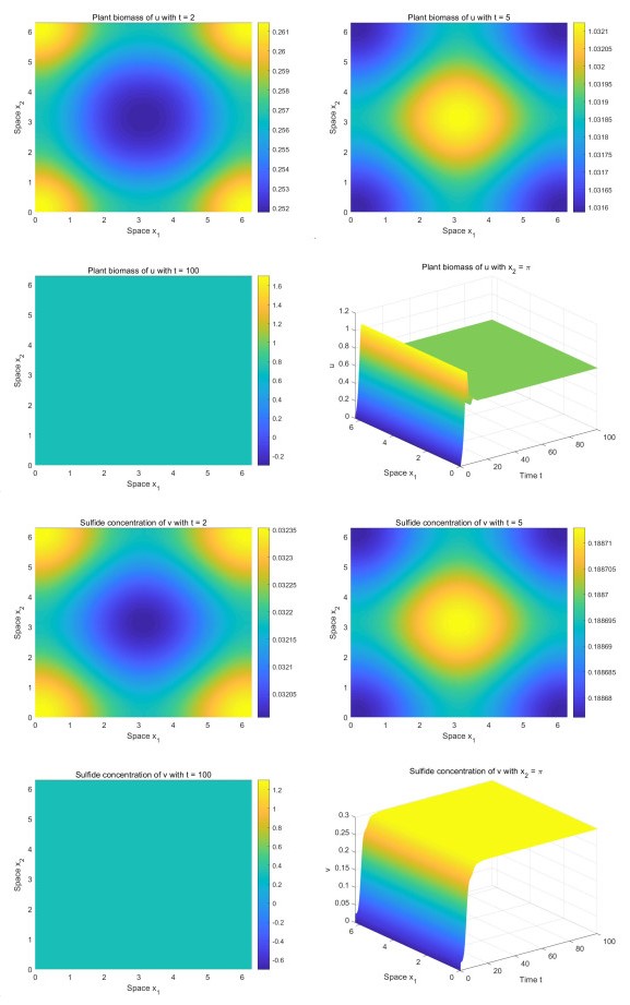
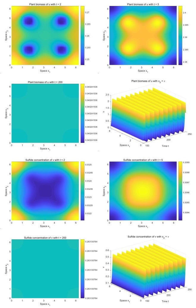
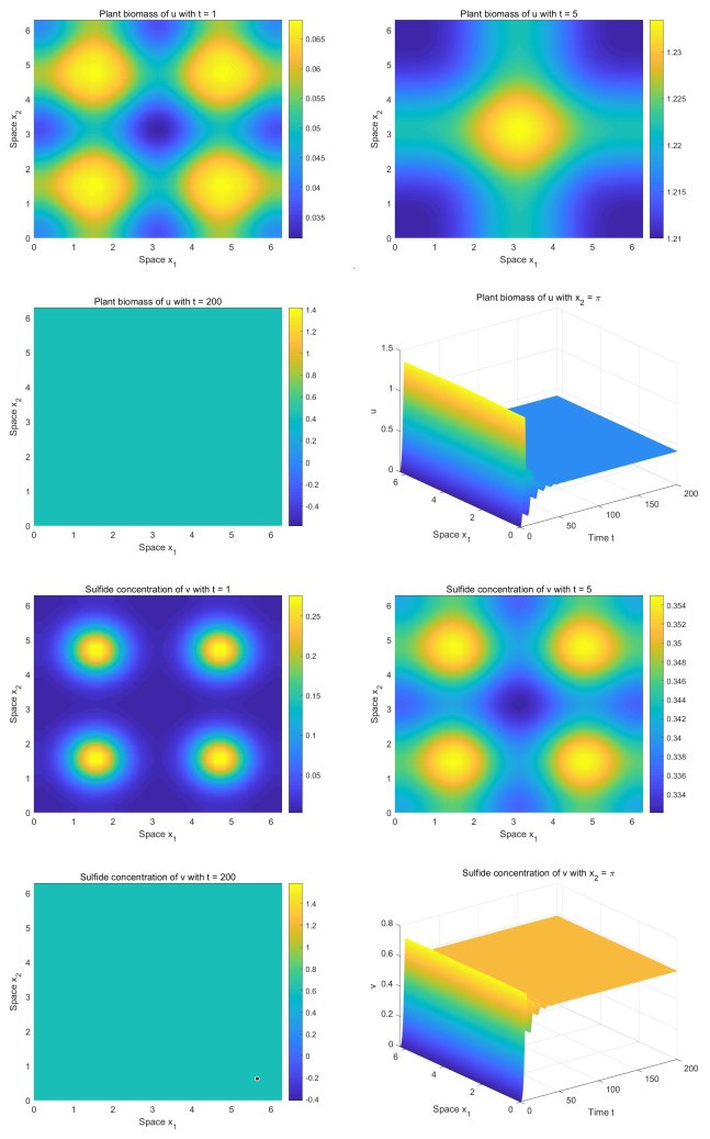
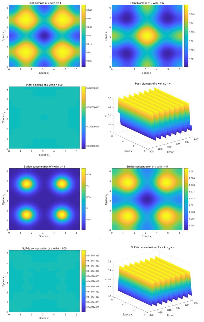
Incorporating the self-regulatory mechanism with time delay to a plant-sulfide feedback system for intertidal salt marshes, we proposed and studied a functional reaction-diffusion model. We analyzed the stability of the positive steady state of the system, and derived the sufficient conditions for the occurrence of Hopf bifurcations. By deriving the normal form on the center manifold, we obtained the formulas determining the properties of the Hopf bifurcations. Our analysis showed that there is a critical value of time delay. When the time delay is greater than the critical value, the system will show asymptotical temporal periodic patterns while the system will display asymptotical spatial homogeneous patterns when the time delay is smaller than the critical value. Our numerical study showed that there are transient fairy circles for any time delay while there are different types of fairy circles and rings in the system. Our results enhance the concept that transient fairy circle patterns in intertidal salt marshes can infer the underlying ecological mechanisms and provide a measure of ecological resilience when the self-regulatory mechanism with time delay is considered.
- transient fairy circle,
- temporal periodic pattern,
- plant-sulfide feedback,
- time delay,
- Hopf bifurcation
Citation: Xin Wei, Jianjun Paul Tian, Jiantao Zhao. Fairy circles and temporal periodic patterns in the delayed plant-sulfide feedback model[J]. Mathematical Biosciences and Engineering, 2024, 21(8): 6783-6806. doi: 10.3934/mbe.2024297

Related Papers:

Abstract

Incorporating the self-regulatory mechanism with time delay to a plant-sulfide feedback system for intertidal salt marshes, we proposed and studied a functional reaction-diffusion model. We analyzed the stability of the positive steady state of the system, and derived the sufficient conditions for the occurrence of Hopf bifurcations. By deriving the normal form on the center manifold, we obtained the formulas determining the properties of the Hopf bifurcations. Our analysis showed that there is a critical value of time delay. When the time delay is greater than the critical value, the system will show asymptotical temporal periodic patterns while the system will display asymptotical spatial homogeneous patterns when the time delay is smaller than the critical value. Our numerical study showed that there are transient fairy circles for any time delay while there are different types of fairy circles and rings in the system. Our results enhance the concept that transient fairy circle patterns in intertidal salt marshes can infer the underlying ecological mechanisms and provide a measure of ecological resilience when the self-regulatory mechanism with time delay is considered.

References

[1]	B. K. van Wesenbeeck, J. Van De Koppel, P. M. J. Herman, T. J. Bouma, Does scale-dependent feedback explain spatial complexity in salt-marsh ecosystems?, Oikos, 117 (2008), 152–159. https://doi.org/10.1111/j.207.0030-1299.16245.x doi: 10.1111/j.207.0030-1299.16245.x
[2]	J. van de Koppel, D. van der Wal, J. P. Bakker, P. M. J Herman, Self-organization and vegetation collapse in salt marsh ecosystems, Am. Nat., 165 (2005), E1–E12. https://doi.org/10.1086/426602 doi: 10.1086/426602
[3]	L. X. Zhao, C. Xu, Z. M. Ge, J. van de Koppel, Q. X. Liu, The shaping role of self-organization: linking vegetation patterning, plant traits and ecosystem functioning, Proc. R. Soc. B, 286 (2019), 20182859. https://doi.org/10.1098/rspb.2018.2859 doi: 10.1098/rspb.2018.2859
[4]	Y. X. Wang, W. T. Li, Spatial patterns of a predator-prey model with Beddington-DeAngelis functional response, Int. J. Bifurcation Chaos, 29 (2019), 1950145. https://doi.org/10.1142/S0218127419501451 doi: 10.1142/S0218127419501451
[5]	X. Guo, J. Wang, Dynamics and pattern formations in diffusive predator-prey models with two prey-taxis, Math. Methods Appl. Sci., 42 (2019), 4197–4212. https://doi.org/10.1002/mma.5639 doi: 10.1002/mma.5639
[6]	D. Song, Y. Song, C. Li, Stability and Turing patterns in a predator-prey model with hunting cooperation and Allee effect in prey population, Int. J. Bifurcation Chaos, 30 (2020), 2050137. https://doi.org/10.1142/S0218127420501370 doi: 10.1142/S0218127420501370
[7]	R. Peng, M. Wang, Pattern formation in the Brusselator system, J. Math. Anal. Appl., 309 (2005), 151–166. https://doi.org/10.1016/j.jmaa.2004.12.026 doi: 10.1016/j.jmaa.2004.12.026
[8]	M. Ghergu, Non-constant steady-state solutions for Brusselator type systems, Nonlinearity, 21 (2008), 2331. https://doi.org/10.1088/0951-7715/21/10/007 doi: 10.1088/0951-7715/21/10/007
[9]	J. Zhou, C. Mu, Pattern formation of a coupled two-cell Brusselator model, J. Math. Anal. Appl., 366 (2010), 679–693. https://doi.org/10.1016/j.jmaa.2009.12.021 doi: 10.1016/j.jmaa.2009.12.021
[10]	M. Wang, Non-constant positive steady states of the Sel'kov model, J. Differ. Equations, 190 (2003), 600-620. https://doi.org/10.1016/S0022-0396(02)00100-6 doi: 10.1016/S0022-0396(02)00100-6
[11]	R. Peng, Qualitative analysis of steady states to the Sel'kov model, J. Differ. Equations, 241 (2007), 386–398. https://doi.org/10.1016/j.jde.2007.06.005 doi: 10.1016/j.jde.2007.06.005
[12]	W. Ni, M. Tang, Turing patterns in the Lengyel-Epstein system for the CIMA reaction, Trans. Am. Math. Soc., 357 (2005), 3953–3969. https://doi.org/10.2307/3845114 doi: 10.2307/3845114
[13]	X. Chen, W. Jiang, Turing-Hopf bifurcation and multi-stable spatio-temporal patterns in the Lengyel-Epstein system, Nonlinear Anal. Real World Appl., 49 (2019), 386–404. https://doi.org/10.1016/j.nonrwa.2019.03.013 doi: 10.1016/j.nonrwa.2019.03.013
[14]	R. Peng, F. Yi, X. Zhao, Spatiotemporal patterns in a reaction-diffusion model with the Degn-Harrison reaction scheme, J. Differ. Equations, 254 (2013), 2465–2498. https://doi.org/10.1016/j.jde.2012.12.009 doi: 10.1016/j.jde.2012.12.009
[15]	S. Li, J. Wu, Y. Dong, Turing patterns in a reaction-diffusion model with the Degn-Harrison reaction scheme, J. Differ. Equations, 259 (2015), 1990–2029. https://doi.org/10.1016/j.jde.2015.03.017 doi: 10.1016/j.jde.2015.03.017
[16]	S. Kfi, M. Rietkerk, C. L. Alados, Y. Pueyo, V. P. Papanastasis, A. ElAich, et al. Spatial vegetation patterns and imminent desertification in Mediterranean arid ecosystems, Nature, 449 (2007), 213–217. https://doi.org/10.1038/nature06111 doi: 10.1038/nature06111
[17]	T. M. Scanlon, K. K. Caylor, S. A. Levin, I. Rodriguez-Iturbe Positive feedbacks promote power-law clustering of Kalahari vegetation, Nature, 449 (2007), 209–212. https://doi.org/10.1038/nature06060 doi: 10.1038/nature06060
[18]	Q. Liu, P. Herman, W. Mooij, J. Huisman, M. Scheffer, H. Olff, et al., Pattern formation at multiple spatial scales drives the resilience of mussel bed ecosystems, Nat. Commun., 5 (2014), 1–7. https://doi.org/10.1038/ncomms6234 doi: 10.1038/ncomms6234
[19]	A. M. Turing, The chemical basis of morphogenesis, in Philosophical Transactions of the Royal Society of London B: Biological Sciences, 237 (1952), 37–72. https://doi.org/10.1098/rstb.1952.0012
[20]	M. Rietkerk, J. van de Koppel, Regular pattern formation in real ecosystems, Trends Ecol. Evol., 23 (2008), 169–175. https://doi.org/10.1016/j.tree.2007.10.013 doi: 10.1016/j.tree.2007.10.013
[21]	N. Juergens, The biological underpinnings of Namib Desert fairy circles, Science, 339 (2013), 1618–1621. https://doi.org/10.1126/science.1222999 doi: 10.1126/science.1222999
[22]	C. Fernandez-Oto, M. Tlidi, D. Escaff, M. G. Clerc, Strong interaction between plants induces circular barren patches: fairy circles, in Philosophical Transactions of the Royal Society A: Mathematical, Physical and Engineering Sciences, 372 (2014), 20140009.
[23]	Y. R. Zelnik, E. Meron, G. Bel, Gradual regime shifts in fairy circles, Proc. Natl. Acad. Sci., 112 (2015), 12327–12331. https://doi.org/10.1073/pnas.1504289112 doi: 10.1073/pnas.1504289112
[24]	S. Getzin, H. Yizhaq, B. Bell, E. Meron, Discovery of fairy circles in Australia supports self-organization theory, Proc. Natl. Acad. Sci., 113 (2016), 3551–3556. https://doi.org/10.1073/pnas.1522130113 doi: 10.1073/pnas.1522130113
[25]	E. Guirado, M. Delgado-Baquerizo, B. M. Benito, F. T. Maestre, The global biogeography and environmental drivers of fairy circles, Proc. Natl. Acad. Sci., 120 (2023), e2304032120. https://doi.org/10.1073/pnas.2304032120 doi: 10.1073/pnas.2304032120
[26]	S. Getzin, S. Holch, J. M. Ottenbreit, H. Yizhaq, K. Wiegand, Spatio-temporal dynamics of fairy circles in Namibia are driven by rainfall and soil infiltrability, Landscape Ecol., 39 (2024), 122. https://doi.org/10.1007/s10980-024-01924-x doi: 10.1007/s10980-024-01924-x
[27]	A. Hastings, K. C. Abbott, K. Cuddington, T. Francis, G. Gellner, Y. C. Lai, et al., Transient phenomena in ecology, Science, 361 (2018), eaat6412. https://doi.org/10.1126/science.aat6412 doi: 10.1126/science.aat6412
[28]	L. Zhao, K. Zhang, K. Siteur, Q. X. Liu, J. van de Koppel, Fairy circles reveal the resilience of self-organized salt marshes, Sci. Adv., 7 (2021), eabe1100. https://doi.org/10.1126/sciadv.abe110 doi: 10.1126/sciadv.abe110
[29]	J. de Fouw, L. Govers, J. van de Koppel, J. van Belzen, W. Dorigo, M. Cheikh, et al., Drought, mutualism breakdown, and landscape-scale degradation of seagrass beds, Curr. Biol., 26 (2016), 1051–1056. https://doi.org/10.1016/j.cub.2016.02.023 doi: 10.1016/j.cub.2016.02.023
[30]	N. Mirlean, C. S. Costa, Geochemical factors promoting die-back gap formation in colonizing patches of Spartina densiflora in an irregularly flooded marsh, Estuarine Coastal Shelf Sci., 189 (2017), 104–114. https://doi.org/10.1016/j.ecss.2017.03.006 doi: 10.1016/j.ecss.2017.03.006
[31]	G. E. Hutchinson, Circular causal systems in ecology, Ann. NY Acad. Sci., 50 (1948), 221–246. https://doi.org/10.1111/j.1749-6632.1948.tb39854.x doi: 10.1111/j.1749-6632.1948.tb39854.x
[32]	J. Wu, Theory and Applications of Partial Functional Differential Equations, Springer, New York, 1996. https://doi.org/10.1007/978-1-4612-4050-1
[33]	K. L. Cooke, Z. Grossman, Discrete delay, distributed delay and stability switches, J. Math. Anal. Appl., 86 (1982), 592–627. https://doi.org/10.1016/0022-247X(82)90243-8 doi: 10.1016/0022-247X(82)90243-8
[34]	S. Ruan, J. Wei, On the zeros of transcendental functions with applications to stability of delay differential equations with two delays, Dyn. Contin. Discrete Impulsive Syst. Ser. A, 10 (2003), 863–874. https://doi.org/10.1093/imammb/18.1.41 doi: 10.1093/imammb/18.1.41
[35]	T. Faria, Normal forms and Hopf bifurcation for partial differential equations with delays, Trans. Am. Math. Soc., 352 (2000), 2217–2238. https://doi.org/10.1090/S0002-9947-00-02280-7 doi: 10.1090/S0002-9947-00-02280-7
[36]	B. D. Hassard, N. D. Kazarinoff, Y. H. Wan, Theory and Applications of Hopf Bifurcation, Cambridge University Press, Cambridge, 1981.

Reader Comments

Your name:*

Email:*
© 2024 the Author(s), licensee AIMS Press. This is an open access article distributed under the terms of the Creative Commons Attribution License (http://creativecommons.org/licenses/by/4.0)