Adaptive boundary control of an axially moving system with large acceleration/deceleration under the input saturation

Yukun Song; Yue Song; Yongjun Wu; Yukun Song; Yue Song; Yongjun Wu

doi:10.3934/mbe.2023810

Mathematical Biosciences and Engineering

2023, Volume 20, Issue 10: 18230-18247. doi: 10.3934/mbe.2023810

Previous Article Next Article

Research article

Adaptive boundary control of an axially moving system with large acceleration/deceleration under the input saturation

College of Science, Liaoning University of Technology, Jinzhou 121001, China

Received: 18 July 2023 Revised: 26 August 2023 Accepted: 12 September 2023 Published: 21 September 2023

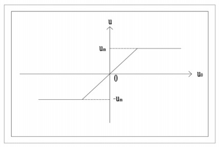
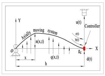
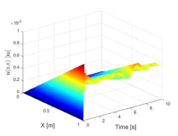
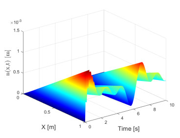
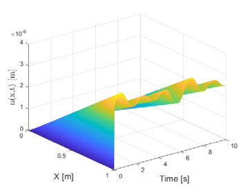
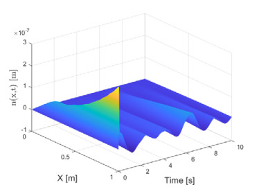
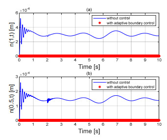
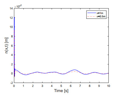
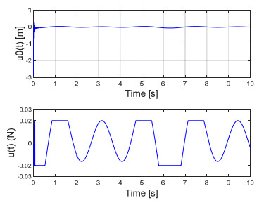
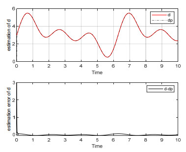
We present the dynamical equation model of the axially moving system, which is expressed through one partial differential equation (PDE) and two ordinary differential equations (ODEs) obtained using the extended Hamilton's principle. In the case of large acceleration/deceleration axially moving system with system parameters uncertainty and input saturation limitation, the combination of Lyapunov theory, S-curve acceleration and deceleration (Sc A/D) and adaptive control techniques adopts auxiliary systems to overcome the saturation limitations of the actuator, thus achieving the purpose of vibration suppression and improving the quality of vibration control. Sc A/D has better flexibility than that of constant speed to ensure the operator performance and diminish the force of impact by tempering the initial acceleration. The designed adaptive control law can avoid the control spillover effect and compensate the system parameters uncertainty. In practice, time-varying boundary interference and distributed disturbance exist in the system. The interference observer is used to track and eliminate the unknown disturbance of the system. The control strategy guarantees the stability of the closed-loop system and the uniform boundedness of all closed-loop states. The numerical simulation results test the effectiveness of the proposed control strategy.
- adaptive boundary control,
- actuator input saturation,
- axially moving system,
- interference observer,
- large acceleration/deceleration
Citation: Yukun Song, Yue Song, Yongjun Wu. Adaptive boundary control of an axially moving system with large acceleration/deceleration under the input saturation[J]. Mathematical Biosciences and Engineering, 2023, 20(10): 18230-18247. doi: 10.3934/mbe.2023810

Related Papers:

Abstract

We present the dynamical equation model of the axially moving system, which is expressed through one partial differential equation (PDE) and two ordinary differential equations (ODEs) obtained using the extended Hamilton's principle. In the case of large acceleration/deceleration axially moving system with system parameters uncertainty and input saturation limitation, the combination of Lyapunov theory, S-curve acceleration and deceleration (Sc A/D) and adaptive control techniques adopts auxiliary systems to overcome the saturation limitations of the actuator, thus achieving the purpose of vibration suppression and improving the quality of vibration control. Sc A/D has better flexibility than that of constant speed to ensure the operator performance and diminish the force of impact by tempering the initial acceleration. The designed adaptive control law can avoid the control spillover effect and compensate the system parameters uncertainty. In practice, time-varying boundary interference and distributed disturbance exist in the system. The interference observer is used to track and eliminate the unknown disturbance of the system. The control strategy guarantees the stability of the closed-loop system and the uniform boundedness of all closed-loop states. The numerical simulation results test the effectiveness of the proposed control strategy.

References

[1]	B. d'Andréa-Novel, J. M. Coron, Exponential stabilization of an overhead crane with flexible cable via a back-stepping approach, Automatica, 36 (2000), 587–593. https://doi.org/10.1016/S0005-1098(99)00182-X doi: 10.1016/S0005-1098(99)00182-X
[2]	M. Krstic, A. Smyshlyaev, Backstepping boundary control for first-order hyperbolic PDEs and application to systems with actuator and sensor delays, Syst. Control Lett., 57 (2008), 750–758. https://doi.org/10.1016/j.sysconle.2008.02.005 doi: 10.1016/j.sysconle.2008.02.005
[3]	Y. Liu, F. Liu, Y. Mei, X. Yao, W. Zhao, Dynamic Modeling and Boundary Control of Flexible Axially Moving System, Springer Nature, 2023. https://doi.org/10.1016/j.sysconle.2008.02.005
[4]	Z. Zhao, Y. Liu, F. Luo, Output feedback boundary control of an axially moving system with input saturation constraint, ISA Trans., 68 (2017), 22–32. https://doi.org/10.1016/j.isatra.2017.02.009 doi: 10.1016/j.isatra.2017.02.009
[5]	L. Hu, F. D. Meglio, R. Vazquez, M. Kristic, Control of homodirectional and general heterodirectional linear coupled hyperbolic PDEs, IEEE Trans. Autom. Control, 61 (2015), 3301–3314. https://doi.org/10.1109/TAC.2015.2512847 doi: 10.1109/TAC.2015.2512847
[6]	D. Pellecchia, N. Vaiana, M. Spizzuoco, G. Serino, L. Rosati, Axial hysteretic behaviour of wire rope isolators: Experiments and modelling, Mater. Des., 225 (2023), 111436. https://doi.org/10.1016/j.matdes.2022.111436 doi: 10.1016/j.matdes.2022.111436
[7]	X. Y. Zhang, L. Tang, Y. J. Liu, Adaptive constraint control for flexible manipulator systems modeled by partial differential equations with dead‐zone input, Int. J. Adapt. Control Signal Process., 35 (2021), 1404–1416. https://doi.org/10.1002/acs.3249 doi: 10.1002/acs.3249
[8]	H. Chen, Y. J. Liu, L. Liu, S. C. Tong, Anti-saturation-based adaptive sliding-mode control for active suspension systems with time-varying vertical displacement and speed constraints, IEEE Trans. Cybern., 52 (2021), 6244–6254. https://doi.org/10.1109/TCYB.2020.3042613 doi: 10.1109/TCYB.2020.3042613
[9]	Y. M. Li, S. C. Tong, Y. J. Liu, T. S. Li, Adaptive fuzzy robust output feedback control of nonlinear systems with unknown dead zones based on a small-gain approach, IEEE Trans. Fuzzy Syst., 22 (2013), 164–176. https://doi.org/10.1109/TFUZZ.2013.2249585 doi: 10.1109/TFUZZ.2013.2249585
[10]	Y. J. Liu, S. C. Tong, Adaptive fuzzy identification and control for a class of nonlinear pure-feedback MIMO systems with unknown dead zones, IEEE Trans. Fuzzy Syst., 24 (2014), 1387–1398. https://doi.org/10.1109/TFUZZ.2014.2360954 doi: 10.1109/TFUZZ.2014.2360954
[11]	Z. Wang, J. Sun, H. Zhang, Stability analysis of T–S fuzzy control system with sampled-dropouts based on time-varying Lyapunov function method, IEEE Trans. Syst. Man Cybern.: Syst., 50 (2018), 2566–2577. https://doi.org/10.1109/TSMC.2018.2822482 doi: 10.1109/TSMC.2018.2822482
[12]	L. Liu, Z. Li, Y. Chen, R. Wang, Disturbance observer-based adaptive intelligent control of marine vessel with position and heading constraint condition related to desired output, IEEE Trans. Neural Networks Learn. Syst., 2022 (2022). https://doi.org/10.1109/TNNLS.2022.3141419 doi: 10.1109/TNNLS.2022.3141419
[13]	J. Sun, C. Guo, L. Liu, Q. H. Shan, Adaptive consensus control of second-order nonlinear multi-agent systems with event-dependent intermittent communications, J. Franklin Inst., 360 (2023), 2289–2306. https://doi.org/10.1016/j.jfranklin.2022.10.045 doi: 10.1016/j.jfranklin.2022.10.045
[14]	K. J. Yang, K. S. Hong, F. Matsuno, Energy-based control of axially translating beams: varying tension, varying speed, and disturbance adaptation, IEEE Trans. Control Syst. Technol., 13 (2005), 1045–1054. https://doi.org/10.1109/TCST.2005.854368 doi: 10.1109/TCST.2005.854368
[15]	Y. H. Feng, Z. Liu, Adaptive vibration iterative learning control of an Euler–Bernoulli beam system with input saturation, IEEE Trans. Syst. Man Cybern.: Syst., 53 (2022), 2469–2477. https://doi.org/10.1109/TSMC.2022.3214571 doi: 10.1109/TSMC.2022.3214571
[16]	S. Zhang, L. Tang, Y. J. Liu, Formation deployment control of multi-agent systems modeled with PDE, Math. Biosci. Eng., 19 (2022), 13541–13559. https://doi.org/10.3934/mbe.2022632 doi: 10.3934/mbe.2022632
[17]	Z. Jing, Y. H. Ma, X. Y. Wu, X. Y. He, Y. B. Sun, Backstepping control for vibration suppression of 2-D Euler–Bernoulli beam based on nonlinear saturation compensator, IEEE Trans. Syst. Man Cybern.: Syst., 53 (2023), 2562–2571. https://doi.org/10.1109/TSMC.2022.3213477 doi: 10.1109/TSMC.2022.3213477
[18]	S. Zhang, Y. T. Dong, Y. C. Ouyang, Z. Yin, K. X. Peng, Adaptive neural control for robotic manipulators with output constraints and uncertainties, IEEE Trans. Neural Networks Learn. Syst., 29 (2018) 5554–5564. https://doi.org/10.1109/TNNLS.2018.2803827 doi: 10.1109/TNNLS.2018.2803827
[19]	Z. Zhao, Y. Liu, W. He, F. Guo, Adaptive boundary control of an axially moving belt system with high acceleration/deceleration, IET Control Theor. Appl., 10 (2016), 1299–1306. https://doi.org/10.1049/iet-cta.2015.0753 doi: 10.1049/iet-cta.2015.0753
[20]	K. J. Yang, K. S. Hong, F. Matsuno, Robust adaptive boundary control of an axially moving string under a spatiotemporally varying tension, J. Sound Vib., 273 (2004), 1007–1029. https://doi.org/10.1016/S0022-460X(03)00519-4 doi: 10.1016/S0022-460X(03)00519-4
[21]	A. Kelleche, N. E. Tatar, Adaptive boundary stabilization of a nonlinear axially moving string, ZAMM J. Appl. Math. Mech., 101 (2021), e202000227. https://doi.org/10.1002/zamm.202000227 doi: 10.1002/zamm.202000227
[22]	B. Tikialine, A. Kelleche, H. A. Tedjani, High-gain adaptive boundary stabilization for an axially moving string subject to unbounded boundary disturbance, Ann. Univ. Craiova-Math. Comput. Sci. Ser., 48 (2021), 112–126. https://doi.org/10.52846/ami.v48i1.1398 doi: 10.52846/ami.v48i1.1398
[23]	C. Y. Wen, J. Zhou, Z. T. Liu, H. Y. Su, Robust adaptive control of uncertain nonlinear systems in the presence of input saturation and external disturbance, IEEE Trans. Autom. Control, 56 (2011), 1672–1678. https://doi.org/10.1109/TAC.2011.2122730 doi: 10.1109/TAC.2011.2122730
[24]	L. H. Chen, W. Zhang, Y. Q. Liu, Modeling of nonlinear oscillations for viscoelastic moving belt using generalized Hamiltons principle, J. Vib. Acoust., 129 (2007), 128–132. https://doi.org/10.1115/1.2346691 doi: 10.1115/1.2346691
[25]	G. H. Hardy, J. E. Littlewood, G. Pólya, Inequalities, Cambridge University Press, 1959.
[26]	A. Smyshlyaev, M. Krstic, Adaptive Control of Parabolic PDEs, Princeton University Press, 2010. https://doi.org/10.1515/9781400835362
[27]	C. D. Rahn, Mechatronic Control of Distributed Noise and Vibration, Springer-Verlag, New York, 2001.
[28]	M. S. De Queiroz, D. M. Dawson, C. D. Rahn, F. Zhang, Adaptive vibration control of an axially moving string, J. Vib. Acoust., 121 (1999), 41–49. https://doi.org/10.1115/1.2893946 doi: 10.1115/1.2893946
[29]	W. He, S. Zhang, S. S. Ge, Robust adaptive control of a thruster assisted position mooring system, Automatica, 50 (2014), 1843–1851. https://doi.org/10.1016/j.automatica.2014.04.023 doi: 10.1016/j.automatica.2014.04.023

Reader Comments

Your name:*

Email:*
© 2023 the Author(s), licensee AIMS Press. This is an open access article distributed under the terms of the Creative Commons Attribution License (http://creativecommons.org/licenses/by/4.0)