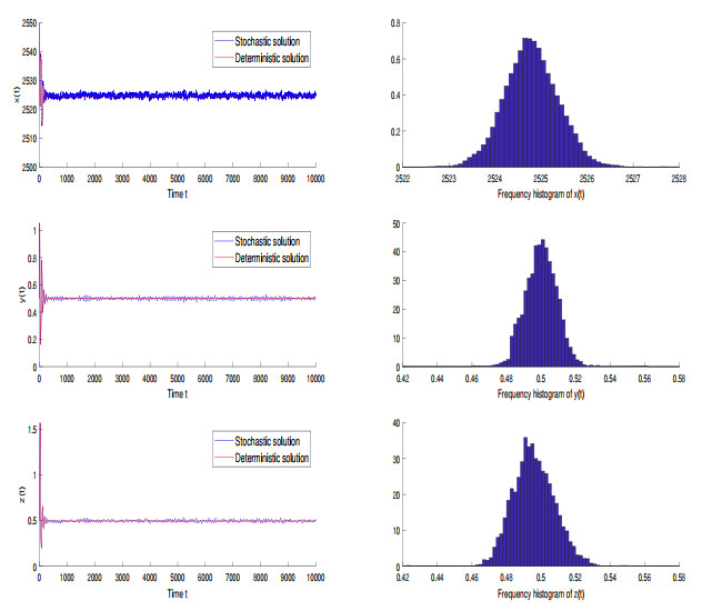
This work examines a stochastic viral infection model with a general distributed delay. We transform the model with weak kernel case into an equivalent system through the linear chain technique. First, we establish that a global positive solution to the stochastic system exists and is unique. We establish the existence of a stationary distribution of a positive solution under the stochastic condition $ R^s > 0 $, also referred to as a stationary solution, by building appropriate Lyapunov functions. Finally, numerical simulation is proved to verify our analytical result and reveals the impact of stochastic perturbations on disease transmission.
Citation: Ying He, Junlong Tao, Bo Bi. Stationary distribution for a three-dimensional stochastic viral infection model with general distributed delay[J]. Mathematical Biosciences and Engineering, 2023, 20(10): 18018-18029. doi: 10.3934/mbe.2023800
This work examines a stochastic viral infection model with a general distributed delay. We transform the model with weak kernel case into an equivalent system through the linear chain technique. First, we establish that a global positive solution to the stochastic system exists and is unique. We establish the existence of a stationary distribution of a positive solution under the stochastic condition $ R^s > 0 $, also referred to as a stationary solution, by building appropriate Lyapunov functions. Finally, numerical simulation is proved to verify our analytical result and reveals the impact of stochastic perturbations on disease transmission.

| [1] |
S. Wang, X. Song, Z. Ge, Dynamics analysis of a delayed viral infection model with immune impairment, Appl. Math. Modell., 35 (2011), 4877–4885. https://doi.org/10.1016/j.apm.2011.03.043 doi: 10.1016/j.apm.2011.03.043

|
| [2] |
C. Bartholdy, J. P. Christensen, D. Wodarz, A. R. Thomsen, Persistent virus infection despite chronic cytotoxic T-lymphocyte activation in Gamma interferon-deficient mice infection with lymphocytic choriomeningitis virus, J. Virol., 74 (2000), 10304–10311. https://doi.org/10.1128/JVI.74.22.10304-10311.2000 doi: 10.1128/JVI.74.22.10304-10311.2000
|
| [3] |
D. Wodarz, J. P. Christensen, A. R. Thomsen, The importance of lytic and nonlytic immune response in viral infections, Trends Immunol., 23 (2002), 194–200. https://doi.org/10.1016/j.apm.2009.11.005 doi: 10.1016/j.apm.2009.11.005
|
| [4] |
Q. Xie, D. Huang, S. Zhang, J. Cao, Analysis of a viral infection model with delayed immune response, Appl. Math. Modell., 34 (2010), 2388–2395. https://doi.org/10.1016/j.apm.2009.11.005 doi: 10.1016/j.apm.2009.11.005
|
| [5] |
C. M. Cluskey, Global stability for an SEIR epidemiological model with varying infectivity and infinite delay, Math. Biosci. Eng., 7 (2009), 603–610. https://doi.org/10.3934/mbe.2009.6.603 doi: 10.3934/mbe.2009.6.603
|
| [6] | Q. Liu, D. Jiang, N. Shi, Stationarity and periodicity of positive solutions to stocahstic SEIR epidemic models with distributed delay, Discrete Contin. Dyn. Syst. B, 22 (2017), 2479–2500. |
| [7] |
X. Sun, W. Zuo, D. Jiang, Unique stationary distribution and ergodicity of a stochastic logistic model with distributed delay, Phys. A, 512 (2018), 864–881. https://doi.org/10.1016/j.physa.2018.08.048 doi: 10.1016/j.physa.2018.08.048
|
| [8] |
T. Caraballo, M. E. Fatini, M. E. Khalifi, Analysis of a stochastic distributed delay epidemic model with relapse and gamma distribution kernel, Chaos Solitons Fractals, 133 (2020), 109643. https://doi.org/10.1016/j.chaos.2020.109643 doi: 10.1016/j.chaos.2020.109643
|
| [9] |
M. Liu, C. Bai, A remark on a stochastic logistic model with Levy jumps, Appl. Math. Comput., 251 (2015), 521–526. https://doi.org/10.1016/j.amc.2014.11.094 doi: 10.1016/j.amc.2014.11.094
|
| [10] |
M. Liu, D. Fan, K. Wang, Stability analysis of a stochastic logistic model with infinite delay, Commun. Commun. Nonlinear Sci. Numer. Simul., 18 (2013), 2289–2294. https://doi.org/10.1016/j.cnsns.2012.12.011 doi: 10.1016/j.cnsns.2012.12.011
|
| [11] |
Y. Liu, Q. Liu, Z. Liu, Dynamical behaviors of a stochastic delay logistic system with impulsive toxicant input in a polluted environment, J. Theor. Biol., 329 (2013), 1–5. https://doi.org/10.1016/j.jtbi.2013.03.005 doi: 10.1016/j.jtbi.2013.03.005
|
| [12] |
C. Lu, X. Ding, Persistence and extinction in general non-autonomous logistic model with delays and stochastic perturbation, Appl. Math. Comput., 229 (2014), 1–15. https://doi.org/10.1016/j.amc.2013.12.042 doi: 10.1016/j.amc.2013.12.042
|
| [13] | Z. Ma, Y. Zhou, J. Wu, Modeling and Dynamic of Infectious Disease, Higher Education Press, Beijing, 2009. |
| [14] |
Y. Wang, D. Jiang, Stationary distribution of an HIV model with general nonlinear incidence rate and stochastic perturbations, J. Franklin Inst., 356 (2019), 6610–6637. https://doi.org/10.1016/j.jfranklin.2019.06.035 doi: 10.1016/j.jfranklin.2019.06.035
|
| [15] | R. Khasminskii, Stochastic Stability of Differential Equations, Springer Science & Business Media, Netherlands, 1980. |
| [16] |
D. Xu, Y. Huang, Z. Yang, Existence theorems for periodic Markov process and stochastic functional differential equations, Discrete Contin. Dyn. Syst., 24 (2009), 1005–1023. https://doi.org/10.3934/dcds.2009.24.1005 doi: 10.3934/dcds.2009.24.1005
|
| [17] |
D. J. Higham, An algorithmic introduction to numerical simulation of stochastic differential equations, SIAM Rev., 43 (2001), 525–546. https://doi.org/10.1137/S0036144500378302 doi: 10.1137/S0036144500378302
|
| [18] |
G. Liu, X. Wang, X. Meng, S. Gao, Extinction and persistence in mean of a novel delay impulsive stochastic infected predator-prey system with jumps, Complexity, 2017 (2017), 1–15. https://doi.org/10.1155/2017/1950970 doi: 10.1155/2017/1950970
|
| [19] |
X. Leng, T. Feng, X. Meng, Stochastic inequalities and applications to dynamics analysis of a novel SIVS epidemic model with jumps, J. Inequalities Appl., 2017 (2017), 138. https://doi.org/10.1186/s13660-017-1418-8 doi: 10.1186/s13660-017-1418-8
|
| [20] |
Y. Shang, Analytical solution for an in-host viral infection model with time-inhomogeneous rates, Acta Phys. Pol. B, 46 (2015), 1567. https://doi.org/10.5506/APhysPolB.46.1567 doi: 10.5506/APhysPolB.46.1567
|
| [21] | Y. Shang, A lie algebra approach to susceptible-infected-susceptible epidemics, Electron. J. Differ. Equations, 233 (2012), 1–7. |
Figures(1)

Ying He, Junlong Tao, Bo Bi. Stationary distribution for a three-dimensional stochastic viral infection model with general distributed delay[J]. Mathematical Biosciences and Engineering, 2023, 20(10): 18018-18029. doi: 10.3934/mbe.2023800


 DownLoad: