Temporal convolution attention model for sepsis clinical assistant diagnosis prediction

Yong Li; Yang Wang; Yong Li; Yang Wang

doi:10.3934/mbe.2023595

Mathematical Biosciences and Engineering

2023, Volume 20, Issue 7: 13356-13378. doi: 10.3934/mbe.2023595

Previous Article Next Article

Research article

Temporal convolution attention model for sepsis clinical assistant diagnosis prediction

Yong Li ,
Yang Wang ^,

College of Computer Science and Engineering, Northwest Normal University, 967 Anning East Road, Lanzhou 730070, China

Academic Editor: Weining Wu

Received: 16 March 2023 Revised: 30 May 2023 Accepted: 05 June 2023 Published: 09 June 2023

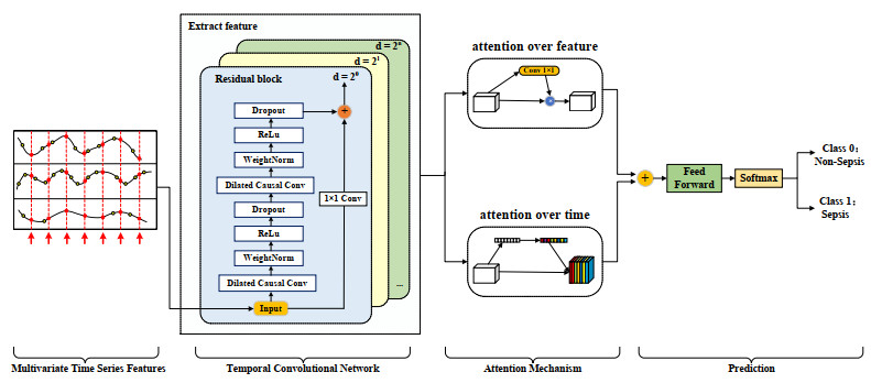
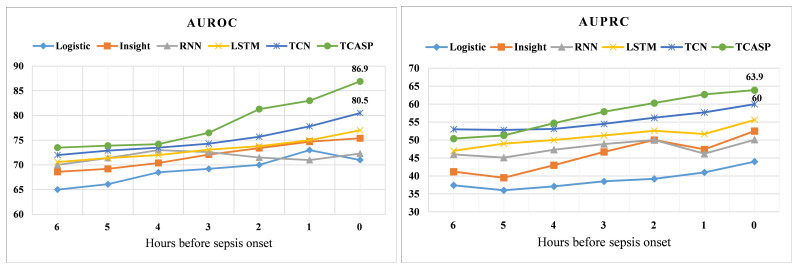
Sepsis is an organ failure disease caused by an infection acquired in an intensive care unit (ICU), which leads to a high mortality rate. Developing intelligent monitoring and early warning systems for sepsis is a key research area in the field of smart healthcare. Early and accurate identification of patients at high risk of sepsis can help doctors make the best clinical decisions and reduce the mortality rate of patients with sepsis. However, the scientific understanding of sepsis remains inadequate, leading to slow progress in sepsis research. With the accumulation of electronic medical records (EMRs) in hospitals, data mining technologies that can identify patient risk patterns from the vast amount of sepsis-related EMRs and the development of smart surveillance and early warning models show promise in reducing mortality. Based on the Medical Information Mart for Intensive Care Ⅲ, a massive dataset of ICU EMRs published by MIT and Beth Israel Deaconess Medical Center, we propose a Temporal Convolution Attention Model for Sepsis Clinical Assistant Diagnosis Prediction (TCASP) to predict the incidence of sepsis infection in ICU patients. First, sepsis patient data is extracted from the EMRs. Then, the incidence of sepsis is predicted based on various physiological features of sepsis patients in the ICU. Finally, the TCASP model is utilized to predict the time of the first sepsis infection in ICU patients. The experiments show that the proposed model achieves an area under the receiver operating characteristic curve (AUROC) score of 86.9% (an improvement of 6.4% ) and an area under the precision-recall curve (AUPRC) score of 63.9% (an improvement of 3.9% ) compared to five state-of-the-art models.
- sepsis assistant diagnosis,
- early prediction,
- electronic medical records,
- temporal convolutional network,
- attention mechanism
Citation: Yong Li, Yang Wang. Temporal convolution attention model for sepsis clinical assistant diagnosis prediction[J]. Mathematical Biosciences and Engineering, 2023, 20(7): 13356-13378. doi: 10.3934/mbe.2023595

Related Papers:

Abstract

Sepsis is an organ failure disease caused by an infection acquired in an intensive care unit (ICU), which leads to a high mortality rate. Developing intelligent monitoring and early warning systems for sepsis is a key research area in the field of smart healthcare. Early and accurate identification of patients at high risk of sepsis can help doctors make the best clinical decisions and reduce the mortality rate of patients with sepsis. However, the scientific understanding of sepsis remains inadequate, leading to slow progress in sepsis research. With the accumulation of electronic medical records (EMRs) in hospitals, data mining technologies that can identify patient risk patterns from the vast amount of sepsis-related EMRs and the development of smart surveillance and early warning models show promise in reducing mortality. Based on the Medical Information Mart for Intensive Care Ⅲ, a massive dataset of ICU EMRs published by MIT and Beth Israel Deaconess Medical Center, we propose a Temporal Convolution Attention Model for Sepsis Clinical Assistant Diagnosis Prediction (TCASP) to predict the incidence of sepsis infection in ICU patients. First, sepsis patient data is extracted from the EMRs. Then, the incidence of sepsis is predicted based on various physiological features of sepsis patients in the ICU. Finally, the TCASP model is utilized to predict the time of the first sepsis infection in ICU patients. The experiments show that the proposed model achieves an area under the receiver operating characteristic curve (AUROC) score of 86.9% (an improvement of 6.4% ) and an area under the precision-recall curve (AUPRC) score of 63.9% (an improvement of 3.9% ) compared to five state-of-the-art models.

References

[1]	M. S. Hari, G. S. Phillips, M. L. Levy, C. W. Seymour, V. X. Liu, C. S. Deutschman, et al., Developing a new definition and assessing new clinical criteria for septic shock: For the third international consensus definitions for sepsis and septic shock (sepsis-3), JAMA, 315 (2016), 775–787. https://doi.org/10.1001/jama.2016.0289 doi: 10.1001/jama.2016.0289
[2]	C. Fleischmann-Struzek, D. M. Goldfarb, P. Schlattmann, L. J. Schlapbach, K. Reinhart, N. Kissoon, The global burden of paediatric and neonatal sepsis: A systematic review, Lancet Respir. Med., 6 (2018), 223–230. https://doi.org/10.1016/S2213-2600(18)30063-8 doi: 10.1016/S2213-2600(18)30063-8
[3]	C. Fleischmann, D. O. Thomas-Rueddel, M. Hartmann, C. S. Hartog, T. Welte, S. Heublein, et al., Hospital incidence and mortality rates of sepsis: An analysis of hospital episode (DRG) statistics in germany from 2007 to 2013, Deutsch. Ärzteblatt Int., 113 (2016), 159. https://doi.org/10.3238%2Farztebl.2016.0159
[4]	S. M. Perman, M. Goyal, D. F. Gaieski, Initial emergency department diagnosis and management of adult patients with severe sepsis and septic shock, Scand. J. Trauma Resusc. Emerg. Med., 20 (2012), 1–11. https://doi.org/10.1186/1757-7241-20-41 doi: 10.1186/1757-7241-20-41
[5]	K. E. Rudd, S. C. Johnson, K. M. Agesa, K. A. Shackelford, D. Tsoi, D. R. Kievlan, et al., Global, regional, and national sepsis incidence and mortality, 1990–2017: Analysis for the global burden of disease study, Lancet, 395 (2020), 200–211. https://doi.org/10.1016/S0140-6736(19)32989-7 doi: 10.1016/S0140-6736(19)32989-7
[6]	M. S. Rangel-Frausto, D. Pittet, M. Costigan, T. Hwang, C. S. Davis, R. P. Wenzel, The natural history of the systemic inflammatory response syndrome (SIRS): A prospective study, Jama, 273 (1995), 117–123. https://doi.org/10.1001/jama.1995.03520260039030 doi: 10.1001/jama.1995.03520260039030
[7]	Á. Castellanos-Ortega, B. Suberviola, L. A. García-Astudillo, M. S. Holanda, F. Ortiz, J. Llorca, et al., Impact of the surviving sepsis campaign protocols on hospital length of stay and mortality in septic shock patients: Results of a three-year follow-up quasi-experimental study, Criti. Care Med., 38 (2010), 1036–1043. https://doi.org/10.1097/CCM.0b013e3181d455b6 doi: 10.1097/CCM.0b013e3181d455b6
[8]	J. K. Sandhu, U. K. Lilhore, M. Poongodi, N. Kaur, S. S. Band, M. Hamdi, et al., Predicting the risk of heart failure based on clinical data, Hum. Centric Comput. Inf. Sci., 12 (2022).
[9]	S. Thandapani, M. I. Mahaboob, C. Iwendi, D. Selvaraj, A. Dumka, M. Rashid, et al., IoMT with deep CNN: Ai-based intelligent support system for pandemic diseases, Electronics, 12 (2023), 424. https://doi.org/10.3390/electronics12020424 doi: 10.3390/electronics12020424
[10]	E. M. Onyema, S. Balasubaramanian, S. K. Suguna, C. Iwendi, B. S. Prasad, C. D. Edeh, Remote monitoring system using slow-fast deep convolution neural network model for identifying anti-social activities in surveillance applications, Meas. Sensors, 27 (2023), 100718. https://doi.org/10.1016/j.measen.2023.100718 doi: 10.1016/j.measen.2023.100718
[11]	H. J. Kam, H. Y. Kim, Learning representations for the early detection of sepsis with deep neural networks, Comput. Biol. Med., 89 (2017), 248–255. https://doi.org/10.1016/j.compbiomed.2017.08.015 doi: 10.1016/j.compbiomed.2017.08.015
[12]	M. A. Reyna, C. Josef, S. Seyedi, R. Jeter, S. P. Shashikumar, M. B. Westover, et al., Early prediction of sepsis from clinical data: The physionet/computing in cardiology challenge 2019, in 2019 Computing in Cardiology (CinC), (2019), 1–4. https://doi.org/10.22489/CinC.2019.412
[13]	S. Nemati, A. Holder, F. Razmi, M. D. Stanley, G. D. Clifford, T. G. Buchman, An interpretable machine learning model for accurate prediction of sepsis in the ICU, Crit. Care Med., 46 (2018), 547. https://doi.org/10.1097%2FCCM.0000000000002936
[14]	E. Sheetrit, N. Nissim, D. Klimov, Y. Shahar, Temporal probabilistic profiles for sepsis prediction in the ICU, in Proceedings of the 25th ACM SIGKDD International Conference on Knowledge Discovery & Data Mining, (2019), 2961–2969. https://doi.org/10.1145/3292500.3330747
[15]	L. M. Fleuren, T. L. Klausch, C. L. Zwager, L. J. Schoonmade, T. Guo, L. F. Roggeveen, et al., Machine learning for the prediction of sepsis: A systematic review and meta-analysis of diagnostic test accuracy, Intensive Care Med., 46 (2020), 383–400. https://doi.org/10.1007/s00134-019-05872-y doi: 10.1007/s00134-019-05872-y
[16]	A. Wong, E. Otles, J. P. Donnelly, A. Krumm, J. McCullough, O. DeTroyer-Cooley, et al., External validation of a widely implemented proprietary sepsis prediction model in hospitalized patients, JAMA Int. Med., 181 (2021), 1065–1070. https://doi.org/10.1001/jamainternmed.2021.2626 doi: 10.1001/jamainternmed.2021.2626
[17]	K. Rahmani, R. Thapa, P. Tsou, S. C. Chetty, G. Barnes, C. Lam, et al., Assessing the effects of data drift on the performance of machine learning models used in clinical sepsis prediction, Int. J. Med. Inf., 173 (2023), 104930. https://doi.org/10.1016/j.ijmedinf.2022.104930 doi: 10.1016/j.ijmedinf.2022.104930
[18]	R. C. Bone, R. A. Balk, F. B. Cerra, R. P. Dellinger, A. M. Fein, W. A. Knaus, et al., Definitions for sepsis and organ failure and guidelines for the use of innovative therapies in sepsis, Chest, 101 (1992), 1644–1655. https://doi.org/10.1378/chest.101.6.1644 doi: 10.1378/chest.101.6.1644
[19]	J. L. Vincent, R. Moreno, J. Takala, S. Willatts, A. De Mendonça, H. Bruining, et al., The sofa (sepsis-related organ failure assessment) score to describe organ dysfunction/failure: On behalf of the working group on sepsis-related problems of the european society of intensive care medicine (see contributors to the project in the appendix), 1996. Available from: http://pirasoa.iavante.es/pluginfile.php/4037/mod_label/intro/18.%20Vincent%201996.pdf.
[20]	C. Stenhouse, S. Coates, M. Tivey, P. Allsop, T. Parker, Prospective evaluation of a modified early warning score to aid earlier detection of patients developing critical illness on a general surgical ward, Br. J. Anaesth., 84 (2000), 663. https://doi.org/10.1093/bja/84.5.663 doi: 10.1093/bja/84.5.663
[21]	O. A. Usman, A. A. Usman, M. A. Ward, Comparison of SIRS, qSOFA, and NEWS for the early identification of sepsis in the emergency department, Am. J. Emerg. Med., 37 (2019), 1490–1497. https://doi.org/10.1016/j.ajem.2018.10.058 doi: 10.1016/j.ajem.2018.10.058
[22]	A. E. Johnson, J. Aboab, J. D. Raffa, T. J. Pollard, R. O. Deliberato, L. A. Celi, et al., A comparative analysis of sepsis identification methods in an electronic database, Crit. Care Med., 46 (2018), 494. https://doi.org/10.1097%2FCCM.0000000000002965
[23]	S. Van der Woude, F. Van Doormaal, B. Hutten, F. Nellen, F. Holleman, Classifying sepsis patients in the emergency department using SIRS, qSOFA or MEWS, Neth. J. Med., 76 (2018), 158–166.
[24]	K. E. Henry, D. N. Hager, P. J. Pronovost, S. Saria, A targeted real-time early warning score (TREWScore) for septic shock, Sci. Transl. Med., 7 (2015), 299ra122. https://doi.org/10.1126/scitranslmed.aab3719 doi: 10.1126/scitranslmed.aab3719
[25]	S. Horng, D. A. Sontag, Y. Halpern, Y. Jernite, N. I. Shapiro, L. A. Nathanson, Creating an automated trigger for sepsis clinical decision support at emergency department triage using machine learning, PloS One, 12 (2017), e0174708. https://doi.org/10.1371/journal.pone.0174708 doi: 10.1371/journal.pone.0174708
[26]	S. Nemati, A. Holder, F. Razmi, M. D. Stanley, G. D. Clifford, T. G. Buchman, An interpretable machine learning model for accurate prediction of sepsis in the ICU, Crit. Care Med., 46 (2018), 547. https://doi.org/10.1097%2FCCM.0000000000002936
[27]	N. Wu, B. Green, X. Ben, S. O'Banion, Deep transformer models for time series forecasting: The influenza prevalence case, preprint, arXiv: 2001.08317. https://doi.org/10.48550/arXiv.2001.08317
[28]	H. Zhou, S. Zhang, J. Peng, S. Zhang, J. Li, H. Xiong, et al., Informer: Beyond efficient transformer for long sequence time-series forecasting, 35 (2021), 11106–11115. https://doi.org/10.1609/aaai.v35i12.17325
[29]	S. S. Rangapuram, M. W. Seeger, J. Gasthaus, L. Stella, Y. Wang, T. Januschowski, Deep state space models for time series forecasting, Adv. Neural Inf. Process. Syst., 2018 (2018), 31.
[30]	C. Lin, Y. Zhang, J. Ivy, M. Capan, R. Arnold, J. M. Huddleston, et al., Early diagnosis and prediction of sepsis shock by combining static and dynamic information using convolutional-LSTM, 2018 (2018), 219–228. https://doi.org/10.1109/ICHI.2018.00032
[31]	S. Baral, A. Alsadoon, P. Prasad, S. Al Aloussi, O. H. Alsadoon, A novel solution of using deep learning for early prediction cardiac arrest in sepsis patient: Enhanced bidirectional long short-term memory (LSTM), Multimedia Tools Appl., 80 (2021), 32639–32664. https://doi.org/10.1007/s11042-021-11176-5 doi: 10.1007/s11042-021-11176-5
[32]	A. Rafiei, A. Rezaee, F. Hajati, S. Gheisari, M. Golzan, SSP: Early prediction of sepsis using fully connected lstm-cnn model, Comput. Biol. Med., 128 (2021), 104110. https://doi.org/10.1016/j.compbiomed.2020.104110 doi: 10.1016/j.compbiomed.2020.104110
[33]	M. Saqib, Y. Sha, M. D. Wang, Early prediction of sepsis in EMR records using traditional ML techniques and deep learning LSTM networks, in 2018 40th Annual International Conference of the IEEE Engineering in Medicine and Biology Society (EMBC), (2018), 4038–4041. https://doi.org/10.1109/EMBC.2018.8513254
[34]	D. Bahdanau, K. Cho, Y. Bengio, Neural machine translation by jointly learning to align and translate, preprint, arXiv: 1409.0473. https://doi.org/10.48550/arXiv.1409.0473
[35]	E. Choi, M. T. Bahadori, J. Sun, J. Kulas, A. Schuetz, W. Stewart, Retain: An interpretable predictive model for healthcare using reverse time attention mechanism, Adv. Neural Inf. Process. Syst., 2016 (2016), 29.
[36]	M. Usama, B. Ahmad, W. Xiao, M. S. Hossain, G. Muhammad, Self-attention based recurrent convolutional neural network for disease prediction using healthcare data, Comput. Methods Programs Biomed., 190 (2020), 05191. https://doi.org/10.1016/j.cmpb.2019.105191 doi: 10.1016/j.cmpb.2019.105191
[37]	W. Lan, X. Wu, Q. Chen, W. Peng, J. Wang, Y. P. Chen, GANLDA: Graph attention network for lncrna-disease associations prediction, Neurocomputing, 469 (2022), 384–393. https://doi.org/10.1016/j.neucom.2020.09.094 doi: 10.1016/j.neucom.2020.09.094
[38]	L. Lin, B. Xu, W. Wu, T. W. Richardson, E. A. Bernal, Medical time series classification with hierarchical attention-based temporal convolutional networks: A case study of myotonic dystrophy diagnosis, in CVPR Workshops, (2019), 83–86.
[39]	E. V. Bonilla, K. Chai, C. Williams, Multi-task gaussian process prediction, Adv. Neural Inf. Proces. Syst., 2007 (2007), 20.
[40]	J. Hu, L. Shen, G. Sun, Squeeze-and-excitation networks, in Proceedings of the IEEE Conference on Computer Vision and Pattern Recognition (CVPR), 2018.
[41]	A. E. Johnson, T. J. Pollard, L. Shen, L. W. H. Lehman, M. Feng, M. Ghassemi, et al., MIMIC-Ⅲ, a freely accessible critical care database, Sci. Data, 3 (2016), 1–9. https://doi.org/10.1038/sdata.2016.35 doi: 10.1038/sdata.2016.35
[42]	F. S. De Menezes, G. R. Liska, M. A. Cirillo, M. J. Vivanco, Data classification with binary response through the boosting algorithm and logistic regression, Exp. Syst. Appl., 69 (2017), 62–73. https://doi.org/10.1016/j.eswa.2016.08.014 doi: 10.1016/j.eswa.2016.08.014
[43]	J. S. Calvert, D. A. Price, U. K. Chettipally, C. W. Barton, M. D. Feldman, J. L. Hoffman, et al., A computational approach to early sepsis detection, Comput. Biol. Med., 74 (2016), 69–73. https://doi.org/10.1016/j.compbiomed.2016.05.003 doi: 10.1016/j.compbiomed.2016.05.003
[44]	J. Futoma, S. Hariharan, K. Heller, M. Sendak, N. Brajer, M. Clement, et al., An improved multi-output gaussian process rnn with real-time validation for early sepsis detection, in Machine Learning for Healthcare Conference, (2017), 243–254.
[45]	K. Greff, R. K. Srivastava, J. Koutník, B. R. Steunebrink, J. Schmidhuber, LSTM: A search space odyssey, IEEE Trans. Neural Networks Learn. Syst., 28 (2016), 2222–2232. https://doi.org/10.1109/TNNLS.2016.2582924 doi: 10.1109/TNNLS.2016.2582924
[46]	M. Moor, M. Horn, B. Rieck, D. Roqueiro, K. Borgwardt, Early recognition of sepsis with gaussian process temporal convolutional networks and dynamic time warping, in Machine Learning for Healthcare Conference, (2019), 2–26.

Reader Comments

Your name:*

Email:*
© 2023 the Author(s), licensee AIMS Press. This is an open access article distributed under the terms of the Creative Commons Attribution License (http://creativecommons.org/licenses/by/4.0)