The high pace emergence in advanced software systems, low-cost hardware and decentralized cloud computing technologies have broadened the horizon for vision-based surveillance, monitoring and control. However, complex and inferior feature learning over visual artefacts or video streams, especially under extreme conditions confine majority of the at-hand vision-based crowd analysis and classification systems. Retrieving event-sensitive or crowd-type sensitive spatio-temporal features for the different crowd types under extreme conditions is a highly complex task. Consequently, it results in lower accuracy and hence low reliability that confines existing methods for real-time crowd analysis. Despite numerous efforts in vision-based approaches, the lack of acoustic cues often creates ambiguity in crowd classification. On the other hand, the strategic amalgamation of audio-visual features can enable accurate and reliable crowd analysis and classification. Considering it as motivation, in this research a novel audio-visual multi-modality driven hybrid feature learning model is developed for crowd analysis and classification. In this work, a hybrid feature extraction model was applied to extract deep spatio-temporal features by using Gray-Level Co-occurrence Metrics (GLCM) and AlexNet transferrable learning model. Once extracting the different GLCM features and AlexNet deep features, horizontal concatenation was done to fuse the different feature sets. Similarly, for acoustic feature extraction, the audio samples (from the input video) were processed for static (fixed size) sampling, pre-emphasis, block framing and Hann windowing, followed by acoustic feature extraction like GTCC, GTCC-Delta, GTCC-Delta-Delta, MFCC, Spectral Entropy, Spectral Flux, Spectral Slope and Harmonics to Noise Ratio (HNR). Finally, the extracted audio-visual features were fused to yield a composite multi-modal feature set, which is processed for classification using the random forest ensemble classifier. The multi-class classification yields a crowd-classification accurac12529y of (98.26%), precision (98.89%), sensitivity (94.82%), specificity (95.57%), and F-Measure of 98.84%. The robustness of the proposed multi-modality-based crowd analysis model confirms its suitability towards real-world crowd detection and classification tasks.
Citation: H. Y. Swathi, G. Shivakumar. Audio-visual multi-modality driven hybrid feature learning model for crowd analysis and classification[J]. Mathematical Biosciences and Engineering, 2023, 20(7): 12529-12561. doi: 10.3934/mbe.2023558
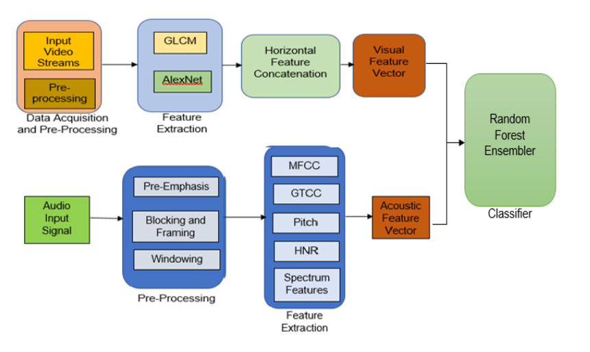
The high pace emergence in advanced software systems, low-cost hardware and decentralized cloud computing technologies have broadened the horizon for vision-based surveillance, monitoring and control. However, complex and inferior feature learning over visual artefacts or video streams, especially under extreme conditions confine majority of the at-hand vision-based crowd analysis and classification systems. Retrieving event-sensitive or crowd-type sensitive spatio-temporal features for the different crowd types under extreme conditions is a highly complex task. Consequently, it results in lower accuracy and hence low reliability that confines existing methods for real-time crowd analysis. Despite numerous efforts in vision-based approaches, the lack of acoustic cues often creates ambiguity in crowd classification. On the other hand, the strategic amalgamation of audio-visual features can enable accurate and reliable crowd analysis and classification. Considering it as motivation, in this research a novel audio-visual multi-modality driven hybrid feature learning model is developed for crowd analysis and classification. In this work, a hybrid feature extraction model was applied to extract deep spatio-temporal features by using Gray-Level Co-occurrence Metrics (GLCM) and AlexNet transferrable learning model. Once extracting the different GLCM features and AlexNet deep features, horizontal concatenation was done to fuse the different feature sets. Similarly, for acoustic feature extraction, the audio samples (from the input video) were processed for static (fixed size) sampling, pre-emphasis, block framing and Hann windowing, followed by acoustic feature extraction like GTCC, GTCC-Delta, GTCC-Delta-Delta, MFCC, Spectral Entropy, Spectral Flux, Spectral Slope and Harmonics to Noise Ratio (HNR). Finally, the extracted audio-visual features were fused to yield a composite multi-modal feature set, which is processed for classification using the random forest ensemble classifier. The multi-class classification yields a crowd-classification accurac12529y of (98.26%), precision (98.89%), sensitivity (94.82%), specificity (95.57%), and F-Measure of 98.84%. The robustness of the proposed multi-modality-based crowd analysis model confirms its suitability towards real-world crowd detection and classification tasks.

| [1] |
J. C. S. Jacques Junior, S. R. Musse, C. R. Jung, Crowd analysis using computer vision techniques, IEEE Signal Process. Mag., 27 (2010), 66–77. https://doi.org/10.1109/MSP.2010.937394 doi: 10.1109/MSP.2010.937394

|
| [2] |
Z. Jie, D. Gao, D. Zhang, Moving vehicle detection for automatic traffic monitoring, vehicular technology, IEEE Trans. Veh. Technol., 56 (2007), 51–59. https://doi.org/10.1109/TVT.2006.883735 doi: 10.1109/TVT.2006.883735
|
| [3] | H. Qiu, X. Liu, S. Rallapalli, A. J. Bency, K. Chan, R. Urgaonkar, et al., Kestrel: Video analytics for augmented multi-camera vehicle tracking, in 2018 IEEE/ACM Third International Conference on Internet-of-Things Design and Implementation (IoTDI), IEEE, Orlando, FL, (2018), 48–59. https://doi.org/10.1109/IoTDI.2018.00015 |
| [4] | R. Mehran, A. Oyama, M. Shah, Abnormal crowd behavior detection using social force model, in 2009 IEEE Conference on Computer Vision and Pattern Recognition, IEEE, (2009), 935–942. https://doi.org/10.1109/CVPR.2009.5206641 |
| [5] |
D. Y. Chen, P. C. Huang, Motion-based unusual event detection in human crowds, J. Visual Commun. Image Represent., 22 (2011), 178–186. https://doi.org/10.1016/j.jvcir.2010.12.004 doi: 10.1016/j.jvcir.2010.12.004
|
| [6] |
C. C. Loy, T. Xiang, S. Gong, Detecting and discriminating behavioural anomalies, Pattern Recognit., 44 (2011), 117–132. https://doi.org/10.1016/j.patcog.2010.07.023 doi: 10.1016/j.patcog.2010.07.023
|
| [7] | P. C. Ribeiro, R. Audigier, Q. C. Pham, RIMOC, a feature to discriminate unstructured motions: Application to violence detection for video-surveillance, Comput. Vision Image Understanding, (2016), 1–23. https://doi.org/10.1016/j.cviu.2015.11.001 |
| [8] |
Y. Benabbas, N. Ihaddadene, C. Djeraba, Motion pattern extraction and event detection for automatic visual surveillance, EURASIP J. Image Video Process., 2011 (2011), 1–7. https://doi.org/10.1155/2011/163682 doi: 10.1155/2011/163682
|
| [9] |
B. Krausz, C. Bauckhage, Loveparade 2010: Automatic video analysis of a crowd disaster, Comput. Vision Image Understanding, 116 (2012), 307–319. https://doi.org/10.1016/j.cviu.2011.08.006 doi: 10.1016/j.cviu.2011.08.006
|
| [10] | V. Kaltsa, A. Briassouli, I. Kompatsiaris, M. G. Strintzis, Timely, robust crowd event characterization, in 19th IEEE International Conference on Image Processing, IEEE, (2012), 2697–2700. https://doi.org/10.1109/ICIP.2012.6467455 |
| [11] | Y. Zhang, L. Qiny, H. Yao, P. Xu, Q. Huang, Beyond particle flow: Bag of trajectory graphs for dense crowd event recognition, in IEEE International Conference on Image Processing, ICIP, 2013. https://doi.org/10.1109/ICIP.2013.6738737 |
| [12] | W. Choi, S. Savarese, A unified framework for multi-target tracking and collective activity recognition, in Computer Vision-ECCV 2012, (2012), 215–230. https://doi.org/10.1007/978-3-642-33765-9_16 |
| [13] | M. Hu, S. Ali, M. Shah, Learning motion patterns in crowded scenes using motion flow field, in 2008 19th International Conference on Pattern Recognition, (2008), 1–5. https://doi.org/10.1109/ICPR.2008.4761183 |
| [14] | S. Ali, M. Shah, A lagrangian particle dynamics approach for crowd flow segmentation and stability analysis, in 2007 IEEE Conference on Computer Vision and Pattern Recognition, CVPR, 2007. https://doi.org/10.1109/CVPR.2007.382977 |
| [15] | C. C. Loy, T. Xiang, S. Gong, Modelling multi-object activity by gaussian processes, in Proceedings of the British Machine Vision Conference, BMVC, 2009. |
| [16] |
A. S. Rao, J. Gubbi, S. Marusic, M. Palaniswami, Crowd event detection on optical flow manifolds, IEEE Trans. Cybern., 46 (2016), 1524–1537. https://doi.org/10.1109/TCYB.2015.2451136 doi: 10.1109/TCYB.2015.2451136
|
| [17] | H. Mousavi, S. Mohammadi, A. Perina, R. Chellali, V. Murino, Analyzing tracklets for the detection of abnormal crowd behavior, in IEEE Winter Conference on Applications of Computer Vision, (2015), 148–155. https://doi.org/10.1109/WACV.2015.27 |
| [18] |
H. Fradi, J. L. Dugelay, Spatial and temporal variations of feature tracks for crowd behavior analysis, J. Multimodal User Interface, 10 (2016), 307–317. https://doi.org/10.1007/s12193-015-0179-2 doi: 10.1007/s12193-015-0179-2
|
| [19] | Y. Zhao, Z. Li, X. Chen, Y. Chen, Mobile crowd sensing service platform for social security incidents in edge computing, in 2018 IEEE International Conference on Internet of Things (iThings) and IEEE Green Computing and Communications (GreenCom) and IEEE Cyber, Physical and Social Computing (CPSCom) and IEEE Smart Data (SmartData), (2018), 568–574. https://doi.org/10.1109/Cybermatics_2018.2018.00118 |
| [20] |
Y. Yuan, J. Fang, Q. Wang, Online anomaly detection in crowd scenes via structure analysis, IEEE Trans. Cybern., 45 (2015), 548–561. https://doi.org/10.1109/TCYB.2014.2330853 doi: 10.1109/TCYB.2014.2330853
|
| [21] | S. Wu, B. E. Moore, M. Shah, Chaotic invariants of Lagrangian particle trajectories for anomaly detection in crowded scenes, in 2010 IEEE Computer Society Conference on Computer Vision and Pattern Recognition, (2010), 2054–2060. https://doi.org/10.1109/CVPR.2010.5539882 |
| [22] | X. Cui, Q. Liu, M. Gao, D. N. Metaxas, Abnormal detection using interaction energy potentials, in Conference on Computer Vision and Pattern Recognition, CVPR, 2011, (2011), 3161–3167. https://doi.org/10.1109/CVPR.2011.5995558 |
| [23] |
S. Cho, H. Kang, Abnormal behavior detection using hybrid agents in crowded scenes, Pattern Recognit. Lett., 44 (2014), 64–70. https://doi.org/10.1016/j.patrec.2013.11.017 doi: 10.1016/j.patrec.2013.11.017
|
| [24] | E. de-la-Calle-Silos, I. González-Díaz, E. Díaz-de-María, Mid-level feature set for specific event and anomaly detection in crowded scenes, in 2013 IEEE International Conference on Image Processing, Melbourne, (2013), 4001–4005. https://doi.org/10.1109/ICIP.2013.6738824 |
| [25] | N. Ihaddadene, C. Djeraba, Real-time crowd motion analysis, in 2008 19th International Conference on Pattern Recognition, (2008), 1–4. https://doi.org/10.1109/ICPR.2008.4761041 |
| [26] | A. N. Shuaibu, A. S. Malik, I. Faye, Behavior representation in visual crowd scenes using space-time features, in 2016 6th International Conference on Intelligent and Advanced Systems (ICIAS), (2016), 1–6. https://doi.org/10.1109/ICIAS.2016.7824073 |
| [27] | R. Hu, Q. Mo, Y. Xie, Y. Xu, J. Chen, Y. Yang, et al., AVMSN: An audio-visual two stream crowd counting framework under low-quality conditions, IEEE Access, 9 (2021), 80500–80510. https://doi.org/10.1109/ACCESS.2021.3074797 |
| [28] | U. Sajid, X. Chen, H. Sajid, T. Kim, G. Wang, Audio-visual transformer based crowd counting, in 2021 IEEE/CVF International Conference on Computer Vision Workshops (ICCVW), (2021), 2249–2259. https://doi.org/10.1109/ICCVW54120.2021.00254 |
| [29] | A. N. Shuaibu, A. S. Malik, I. Faye, Adaptive feature learning CNN for behavior recognition in crowd scene, in 2017 IEEE International Conference on Signal and Image Processing Applications (ICSIPA), Malaysia, (2017), 357–361. https://doi.org/10.1109/ICSIPA.2017.8120636 |
| [30] |
K. Zheng, W. Q. Yan, P. Nand, Video dynamics detection using deep neural networks, IEEE Trans. Emerging Top. Comput. Intell., 2 (2018), 224–234. https://doi.org/10.1109/TETCI.2017.2778716 doi: 10.1109/TETCI.2017.2778716
|
| [31] |
Y. Li, A deep spatio-temporal perspective for understanding crowd behavior, IEEE Trans. Multimedia, 20 (2018), 3289–3297. https://doi.org/10.1109/TMM.2018.2834873 doi: 10.1109/TMM.2018.2834873
|
| [32] | L. F. Borja-Borja, M. Saval-Calvo, J. Azorin-Lopez, A short review of deep learning methods for understanding group and crowd activities, in 2018 International Joint Conference on Neural Networks (IJCNN), Rio de Janeiro, (2018), 1–8. https://doi.org/10.1109/IJCNN.2018.8489692 |
| [33] | B. Mandal, J. Fajtl, V. Argyriou, D. Monekosso, P. Remagnino, Deep residual network with subclass discriminant analysis for crowd behavior recognition, in 2018 25th IEEE International Conference on Image Processing (ICIP), Athens, (2018), 938–942. https://doi.org/10.1109/ICIP.2018.8451190 |
| [34] | A. N. Shuaibu, A. S. Malik, I. Faye, Y. S. Ali, Pedestrian group attributes detection in crowded scenes, in 2017 International Conference on Advanced Technologies for Signal and Image Processing (ATSIP), Fez, (2017), 1–5. https://doi.org/10.1109/ATSIP.2017.8075584 |
| [35] |
F. Solera, S. Calderara, R. Cucchiara, Socially constrained structural learning for groups detection in crowd, IEEE Trans. Pattern Anal. Mach. Intell., 38 (2016), 995–1008. https://doi.org/10.1109/TPAMI.2015.2470658 doi: 10.1109/TPAMI.2015.2470658
|
| [36] |
S. Kim, S. Kwak, B. C. Ko, Fast pedestrian detection in surveillance video based on soft target training of shallow random forest, IEEE Access, 7 (2019), 12415–12426. https://doi.org/10.1109/ACCESS.2019.2892425 doi: 10.1109/ACCESS.2019.2892425
|
| [37] |
S. Din, A. Paul, A. Ahmad, B. B. Gupta, S. Rho, Service orchestration of optimizing continuous features in industrial surveillance using Big Data based fog-enabled Internet of Things, IEEE Access, 6 (2018), 21582–21591. https://doi.org/10.1109/ACCESS.2018.2800758 doi: 10.1109/ACCESS.2018.2800758
|
| [38] |
M. U. K. Khan, H. Park, C. Kyung, Rejecting motion outliers for efficient crowd anomaly detection, IEEE Trans. Inf. Forensics Secur., 14 (2018), 541–556. https://doi.org/10.1109/TIFS.2018.2856189 doi: 10.1109/TIFS.2018.2856189
|
| [39] |
A. N. Shuaibu, I. Faye, Y. Salih Ali, N. Kamel, M. N. Saad, A. S. Malik, Sparse representation for crowd attributes recognition, IEEE Access, 5 (2017), 10422–10433. https://doi.org/10.1109/ACCESS.2017.2708838 doi: 10.1109/ACCESS.2017.2708838
|
| [40] |
C. Riachy, F. Khelifi, A. Bouridane, Video-based person re-identification using unsupervised tracklet matching, IEEE Access, 7 (2019), 20596–20606. https://doi.org/10.1109/ACCESS.2019.2896779 doi: 10.1109/ACCESS.2019.2896779
|
| [41] | H. Fradi, J. Dugelay, Sparse feature tracking for crowd change detection and event recognition, in 2014 22nd International Conference on Pattern Recognition, ICPR, (2014), 4116–4121. https://doi.org/10.1109/ICPR.2014.705 |
| [42] | B. Yogameena, S. Saravana Perumal, N. Packiyaraj, P. Saravanan, Ma-Th algorithm for people count in a dense crowd and their behaviour classification, in 2012 International Conference on Machine Vision and Image Processing (MVIP), Taipei, (2012), 17–20. https://doi.org/10.1109/MVIP.2012.6428750 |
| [43] | R. Mehran, A. Oyama, M. Shah, Abnormal crowd behavior detection using social force model, in 2009 IEEE Conference on Computer Vision and Pattern Recognition, Miami, FL, (2009), 935–942. https://doi.org/10.1109/ICIP.2012.6467453 |
| [44] | X. Zhou, L. Zhang, Abnormal event detection using recurrent neural network, in 2015 International Conference on Computer Science and Applications (CSA), Wuhan, (2015), 222–226. https://doi.org/10.1109/CSA.2015.64 |
| [45] | S. S. Pathan, A. Al-Hamadi, B. Michaelis, Crowd behavior detection by statistical modeling of motion patterns, in 2010 International Conference of Soft Computing and Pattern Recognition, Paris, (2010), 81–86. https://doi.org/10.1109/SOCPAR.2010.5686403 |
| [46] | S. Wang, Z. Miao, Anomaly detection in crowd scene using historical information, in 2010 International Symposium on Intelligent Signal Processing and Communication Systems, Chengdu, (2010), 1–4. https://doi.org/10.1109/ISPACS.2010.5704770 |
| [47] |
P. Wang, W. Hao, Z. Sun, S. Wang, E. Tan, L. Li, et al., Regional detection of traffic congestion using in a large-scale surveillance system via deep residual TrafficNet, IEEE Access, 6 (2018), 68910–68919. https://doi.org/10.1109/ACCESS.2018.2879809 doi: 10.1109/ACCESS.2018.2879809
|
| [48] |
T. P. Nguyen, C. C. Pham, S. V. Ha, J. W. Jeon, Change detection by training a triplet network for motion feature extraction, IEEE Trans. Circuits Syst. Video Technol., 29 (2019), 433–446. https://doi.org/10.1109/TCSVT.2018.2795657 doi: 10.1109/TCSVT.2018.2795657
|
| [49] |
C. Riachy, F. Khelifi, A. Bouridane, Video-based person re-identification using unsupervised tracklet matching, IEEE Access, 7 (2019), 20596–20606. https://doi.org/10.1109/ACCESS.2019.2896779 doi: 10.1109/ACCESS.2019.2896779
|
| [50] |
G. Olague, D. E. Hernández, E. Clemente, M. Chan-Ley, Evolving head tracking routines with brain programming, IEEE Access, 6 (2018), 26254–26270. https://doi.org/10.1109/ACCESS.2018.2831633 doi: 10.1109/ACCESS.2018.2831633
|
| [51] |
Y. Lee, S. Chen, J. Hwang, Y. Hung, An ensemble of invariant features for person reidentification, IEEE Trans. Circuits Syst. Video Technol., 27 (2017), 470–483. https://doi.org/10.1109/TCSVT.2016.2637818 doi: 10.1109/TCSVT.2016.2637818
|
| [52] |
S. Yi, H. Li, X. Wang, Pedestrian behavior modeling from stationary crowds with applications to intelligent surveillance, IEEE Trans. Image Process., 25 (2016), 4354–4368. https://doi.org/10.1109/TIP.2016.2590322 doi: 10.1109/TIP.2016.2590322
|
| [53] |
Bera, S. Kim, D. Manocha, Interactive crowd-behavior learning for surveillance and training, IEEE Comput. Graphics Appl., 36 (2016), 37–45. https://doi.org/10.1109/MCG.2016.113 doi: 10.1109/MCG.2016.113
|
| [54] |
H. Fradi, B. Luvison, Q. C. Pham, Crowd behavior analysis using local mid-level visual descriptors, IEEE Trans. Circuits Syst. Video Technol., 27 (2017), 589–602. https://doi.org/10.1109/TCSVT.2016.2615443 doi: 10.1109/TCSVT.2016.2615443
|
| [55] |
M. Abdar, N. Y. Yen, Design of a universal user model for dynamic crowd preference sensing and decision-making behavior analysis, IEEE Access, 5 (2017), 24842–24852. https://doi.org/10.1109/ACCESS.2017.2735242 doi: 10.1109/ACCESS.2017.2735242
|
| [56] |
X. Zhang, Q. Yu, H. Yu, Physics inspired methods for crowd video surveillance and analysis: A survey, IEEE Access, 6 (2018), 66816–66830. https://doi.org/10.1109/ACCESS.2018.2878733 doi: 10.1109/ACCESS.2018.2878733
|
| [57] |
Y. Zhang, L. Qin, R. Ji, S. Zhao, Q. Huang, J. Luo, Exploring coherent motion patterns via structured trajectory learning for crowd mood modeling, IEEE Trans. Circuits Syst. Video Technol., 27 (2017), 635–648. https://doi.org/10.1109/TCSVT.2016.2593609 doi: 10.1109/TCSVT.2016.2593609
|
| [58] |
W. Liu, R. W. H. Lau, X. Wang, D. Manocha, Exemplar-AMMs: Recognizing Crowd movements from pedestrian trajectories, IEEE Trans. Multimedia, 18 (2016), 2398–2406. https://doi.org/10.1109/TMM.2016.2598091 doi: 10.1109/TMM.2016.2598091
|
| [59] |
C. Chen, Y. Shao, X. Bi, Detection of anomalous crowd behavior based on the acceleration feature, IEEE Sensors J., 15 (2015), 7252–7261. https://doi.org/10.1109/JSEN.2015.2472960 doi: 10.1109/JSEN.2015.2472960
|
| [60] |
V. J. Kok, C. S. Chan, GrCS: Granular computing-based crowd segmentation, IEEE Trans. Cybern., 47 (2017), 1157–11680. https://doi.org/10.1109/TCYB.2016.2538765 doi: 10.1109/TCYB.2016.2538765
|
| [61] |
C. Chen, Y. Shao, Crowd escape behavior detection and localization based on divergent centers, IEEE Sensors J., 15 (2015), 2431–2439. https://doi.org/10.1109/JSEN.2014.2381260 doi: 10.1109/JSEN.2014.2381260
|
| [62] |
Y. Zhang, L. Qin, R. Ji, H. Yao, Q. Huang, Social attribute-aware force model: Exploiting richness of interaction for abnormal crowd detection, IEEE Trans. Circuits Syst. Video Technol., 25 (2015), 1231–1245. https://doi.org/10.1109/TCSVT.2014.2355711 doi: 10.1109/TCSVT.2014.2355711
|
| [63] |
H. Yao, A. Cavallaro, T. Bouwmans, Z. Zhang, Guest Editorial Introduction to the Special Issue on group and crowd behavior analysis for intelligent multicamera video surveillance, IEEE Trans. Circuits Syst. Video Technol., 27 (2017), 405–408. https://doi.org/10.1109/TCSVT.2017.2669658 doi: 10.1109/TCSVT.2017.2669658
|
| [64] |
A. S. Keçeli, A. Kaya, Violent activity detection with transfer learning method, Electron. Lett., 53 (2017), 1047–1048. https://doi.org/10.1049/el.2017.0970 doi: 10.1049/el.2017.0970
|
| [65] |
V. Kaltsa, A. Briassouli, I. Kompatsiaris, L. J. Hadjileontiadis, M. G. Strintzis, Swarm intelligence for detecting interesting events in crowded environments, IEEE Trans. Image Process., 24 (2015), 2153–2166. https://doi.org/10.1109/TIP.2015.2409559 doi: 10.1109/TIP.2015.2409559
|
| [66] | V. H. Roldão Reis, S. J. F. Guimarães, Z. K. Gonçalves do Patrocínio, Dense crowd counting with capsule networks, in 2020 International Conference on Systems, Signals and Image Processing (IWSSIP), (2020), 267–272. https://doi.org/10.1109/IWSSIP48289.2020.9145163 |
| [67] | P. Foggia, A. Saggese, N. Strisciuglio, M. Vento, N. Petkov, Car crashes detection by audio analysis in crowded roads, in 2015 12th IEEE International Conference on Advanced Video and Signal Based Surveillance (AVSS), (2015), 1–6. https://doi.org/10.1109/AVSS.2015.7301731 |
| [68] | S. Duan, X. Wang, X. Yu, Crowded abnormal detection based on mixture of kernel dynamic texture, in 2014 International Conference on Audio, Language and Image Processing, (2014), 931–936. https://doi.org/10.1109/ICALIP.2014.7009931 |
| [69] | Ç. Okuyucu, M. Sert, A. Yazici, Audio feature and classifier analysis for efficient recognition of environmental sounds, in 2013 IEEE International Symposium on Multimedia, (2013), 125–132. https://doi.org/10.1109/ISM.2013.29 |
| [70] | M. Baillie, J. M. Jose, An audio-based sports video segmentation and event detection algorithm, in 2004 Conference on Computer Vision and Pattern Recognition Workshop, (2004), 110. https://doi.org/10.1109/CVPR.2004.298 |
| [71] | M. A. Hossan, S. Memon, M. A. Gregory, A novel approach for MFCC feature extraction, in 2010 4th International Conference on Signal Processing and Communication Systems, (2011), 1–5. https://doi.org/10.1109/ICSPCS.2010.5709752 |
| [72] | T. D. Ganchev, Speaker Recognition, PhD thesis, University of Patras, 2005. |
| [73] |
H. Y. Swathi, G. Shivakumar, Evolutionary computing assisted neural network for crowd behaviour classification, Neuroquantology, 20 (2022), 2848–2855. https://doi.org/10.14704/nq.2022.20.9.NQ44331 doi: 10.14704/nq.2022.20.9.NQ44331
|
| [74] | http://mha.cs.umn.edu/Movies/Crowd-Activity-All.avi |
| [75] | PETS09 dataset, Available from: http://www.cvg.reading.ac.uk/PETS2009/a.html. |
| [76] | M. Marsden, K. McGuinness, S. Little, N. E. O'Connor, Holistic features for real-time crowd behaviour anomaly detection, in 2016 IEEE International Conference on Image Processing (ICIP), Phoenix, AZ, (2016), 918–922. https://doi.org/10.1109/ICIP.2016.7532491 |
| [77] | S. Mohammadi, A. Perina, V. Murino, Violence detection in crowded scenes using substantial derivative, in 2015 12th IEEE International Conference on Advanced Video and Signal Based Surveillance (AVSS), 2015. https://doi.org/10.1109/AVSS.2015.7301787 |
| [78] | H. Mousavi, S. Mohammadi, A. Perina, R. Chellali, V. Murino, Analyzing tracklets for the detection of abnormal crowd behavior, in 2015 IEEE Winter Conference on Applications of Computer Vision, IEEE, (2015), 148–155. https://doi.org/10.1109/WACV.2015.27 |
| [79] | Y. Itcher, T. Hassner, O, Kliper-Gross, Violent flows: Real-time detection of violent crowd behavior, in 2012 IEEE Computer Society Conference on Computer Vision and Pattern Recognition Workshops, 2012. https://doi.org/10.1109/CVPRW.2012.6239348 |
| [80] | H. Mousavi, M. Nabi, H. Kiani, A. Perina, V Murino, Crowd motion monitoring using tracklet-based commotion measure, in 2015 IEEE International Conference on Image Processing (ICIP), IEEE, 2015. https://doi.org/10.1109/ICIP.2015.7351223 |
| [81] | L. Lu, J. He, Z. Xu, Y. Xu, C. Zhang, J. Wang, et al., Crowd behavior understanding through SIOF feature analysis, in 2017 23rd International Conference on Automation and Computing (ICAC), Huddersfield, (2017), 1–6. https://doi.org/10.23919/IConAC.2017.8082086 |


Figures(6) / Tables(4)

H. Y. Swathi, G. Shivakumar. Audio-visual multi-modality driven hybrid feature learning model for crowd analysis and classification[J]. Mathematical Biosciences and Engineering, 2023, 20(7): 12529-12561. doi: 10.3934/mbe.2023558


 DownLoad: