Papillary renal cell carcinoma (PRCC) is a malignant neoplasm of the kidney and is highly interesting due to its increasing incidence. Many studies have shown that the basement membrane (BM) plays an important role in the development of cancer, and structural and functional changes in the BM can be observed in most renal lesions. However, the role of BM in the malignant progression of PRCC and its impact on prognosis has not been fully studied. Therefore, this study aimed to explore the functional and prognostic value of basement membrane-associated genes (BMs) in PRCC patients. We identified differentially expressed BMs between PRCC tumor samples and normal tissue and systematically explored the relevance of BMs to immune infiltration. Moreover, we constructed a risk signature based on these differentially expressed genes (DEGs) using Lasso regression analysis and demonstrated their independence using Cox regression analysis. Finally, we predicted 9 small molecule drugs with the potential to treat PRCC and compared the differences in sensitivity to commonly used chemotherapeutic agents between high and low-risk groups to better target patients for more precise treatment planning. Taken together, our study suggested that BMs might play a crucial role in the development of PRCC, and these results might provide new insights into the treatment of PRCC.
Citation: Yujia Xi, Liying Song, Shuang Wang, Haonan Zhou, Jieying Ren, Ran Zhang, Feifan Fu, Qian Yang, Guosheng Duan, Jingqi Wang. Identification of basement membrane-related prognostic signature for predicting prognosis, immune response and potential drug prediction in papillary renal cell carcinoma[J]. Mathematical Biosciences and Engineering, 2023, 20(6): 10694-10724. doi: 10.3934/mbe.2023474
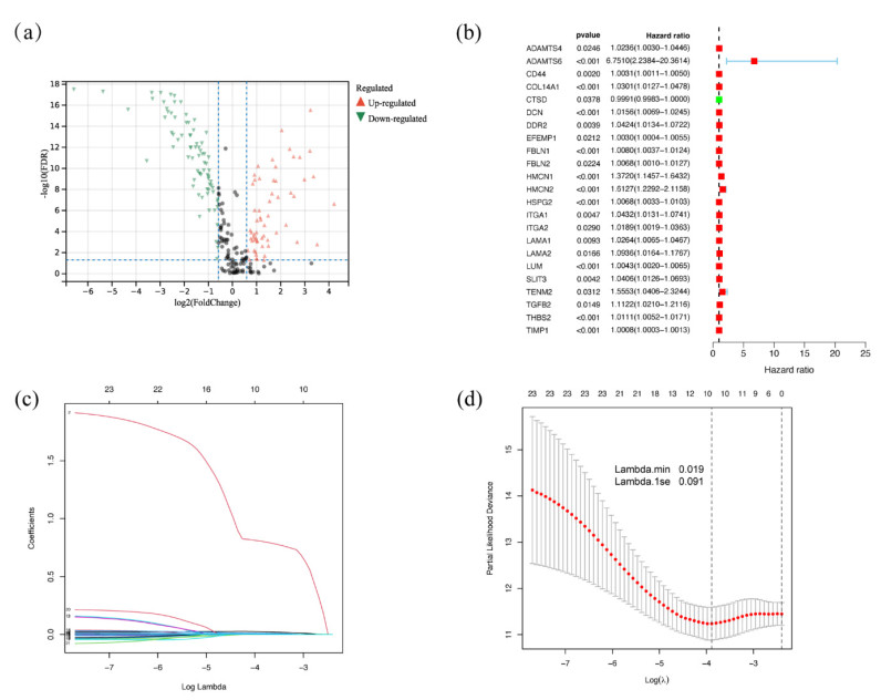
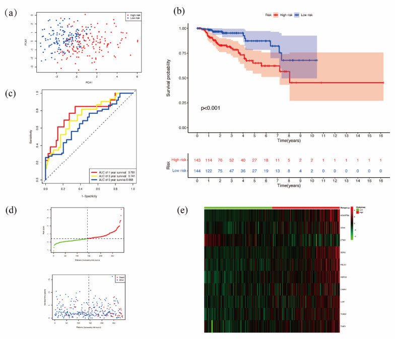
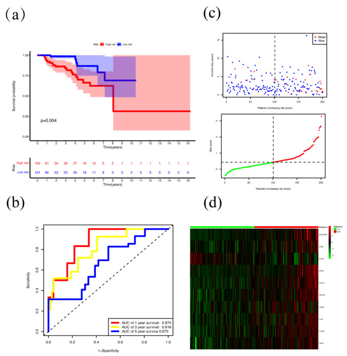
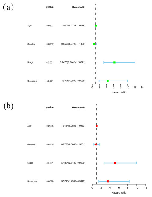
Papillary renal cell carcinoma (PRCC) is a malignant neoplasm of the kidney and is highly interesting due to its increasing incidence. Many studies have shown that the basement membrane (BM) plays an important role in the development of cancer, and structural and functional changes in the BM can be observed in most renal lesions. However, the role of BM in the malignant progression of PRCC and its impact on prognosis has not been fully studied. Therefore, this study aimed to explore the functional and prognostic value of basement membrane-associated genes (BMs) in PRCC patients. We identified differentially expressed BMs between PRCC tumor samples and normal tissue and systematically explored the relevance of BMs to immune infiltration. Moreover, we constructed a risk signature based on these differentially expressed genes (DEGs) using Lasso regression analysis and demonstrated their independence using Cox regression analysis. Finally, we predicted 9 small molecule drugs with the potential to treat PRCC and compared the differences in sensitivity to commonly used chemotherapeutic agents between high and low-risk groups to better target patients for more precise treatment planning. Taken together, our study suggested that BMs might play a crucial role in the development of PRCC, and these results might provide new insights into the treatment of PRCC.

| [1] |
G. Courthod, M. Tucci, M. Di Maio, G. V. Scagliotti, Papillary renal cell carcinoma: A review of the current therapeutic landscape, Crit. Rev. Oncol./Hematol., 96 (2015), 100–112. https://doi.org/10.1016/j.critrevonc.2015.05.008 doi: 10.1016/j.critrevonc.2015.05.008

|
| [2] |
N. Mendhiratta, P. Muraki, A. E. Sisk Jr, B. Shuch, Papillary renal cell carcinoma: Review, Urol. Oncol.: Semin. Orig. Invest., 39 (2021), 327–337. https://doi.org/10.1016/j.urolonc.2021.04.013 doi: 10.1016/j.urolonc.2021.04.013
|
| [3] |
J. Cheng, Z. Han, R. Mehra, W. Shao, M. Cheng, Q. Feng, et al., Computational analysis of pathological images enables a better diagnosis of TFE3 Xp11.2 translocation renal cell carcinoma, Nat. Commun., 11 (2020), 1778. https://doi.org/10.1038/s41467-020-15671-5 doi: 10.1038/s41467-020-15671-5
|
| [4] |
S. Steffens, M. Janssen, F. C. Roos, F. Becker, S. Schumacher, C. Seidel, et al., Incidence and long-term prognosis of papillary compared to clear cell renal cell carcinoma-a multicentre study, Eur. J. Cancer, 48 (2012), 2347–2352. https://doi.org/10.1016/j.ejca.2012.05.002 doi: 10.1016/j.ejca.2012.05.002
|
| [5] |
Q. Chen, L. Cheng, Q. Li, The molecular characterization and therapeutic strategies of papillary renal cell carcinoma, Expert Rev. Anticancer Ther., 19 (2019), 169–175. https://doi.org/10.1080/14737140.2019.1548939 doi: 10.1080/14737140.2019.1548939
|
| [6] |
M. de Vries-Brilland, D. F. McDermott, C. Suárez, T. Powles, M. Gross-Goupil, A. Ravaud, et al., Checkpoint inhibitors in metastatic papillary renal cell carcinoma, Cancer Treat. Rev., 99 (2021), 102228. https://doi.org/10.1016/j.ctrv.2021.102228 doi: 10.1016/j.ctrv.2021.102228
|
| [7] |
R. Reuten, S. Zendehroud, M. Nicolau, L. Fleischhauer, A. Laitala, S. Kiderlen, et al., Basement membrane stiffness determines metastases formation, Nat. Mater., 20 (2021), 892–903. https://doi.org/10.1038/s41563-020-00894-0 doi: 10.1038/s41563-020-00894-0
|
| [8] |
S. E. Wilson, A. Torricelli, G. K. Marino, Corneal epithelial basement membrane: Structure, function and regeneration, Exp. Eye Res., 194 (2020), 108002. https://doi.org/10.1016/j.exer.2020.108002 doi: 10.1016/j.exer.2020.108002
|
| [9] |
N. Khalilgharibi, Y. Mao, To form and function: on the role of basement membrane mechanics in tissue development, homeostasis and disease, Open Biol., 11 (2021), 200360. https://doi.org/10.1098/rsob.200360 doi: 10.1098/rsob.200360
|
| [10] |
F. Kai, A. P. Drain, V. M. Weaver, The extracellular matrix modulates the metastatic journey, Dev. Cell, 49 (2019), 332–346. https://doi.org/10.1016/j.devcel.2019.03.026 doi: 10.1016/j.devcel.2019.03.026
|
| [11] |
R. W. Naylor, M. Morais, R. Lennon, Complexities of the glomerular basement membrane, Nat. Rev. Nephrol., 17 (2021), 112–127. https://doi.org/10.1038/s41581-020-0329-y doi: 10.1038/s41581-020-0329-y
|
| [12] |
R. Jayadev, M. Morais, J. M. Ellingford, S. Srinivasan, R. W. Naylor, C. Lawless, et al., A basement membrane discovery pipeline uncovers network complexity, regulators, and human disease associations, Sci. Adv., 8 (2022), 2265. https://doi.org/10.1126/sciadv.abn2265 doi: 10.1126/sciadv.abn2265
|
| [13] |
D. Szklarczyk, A. L. Gable, K. C. Nastou, D. Lyon, R. Kirsch, S. Pyysalo, et al., The STRING database in 2021: customizable protein-protein networks, and functional characterization of user-uploaded gene/measurement sets, Nucleic Acids Res., 49 (2021), 605–612. https://doi.org/10.1093/nar/gkaa1074 doi: 10.1093/nar/gkaa1074
|
| [14] |
D. Szklarczyk, A. L. Gable, D. Lyon, A. Junge, S. Wyder, J. Huerta-Cepas, et al., STRING v11: protein-protein association networks with increased coverage, supporting functional discovery in genome-wide experimental datasets, Nucleic Acids Res., 47 (2019), 607–613. https://doi.org/10.1093/nar/gky1131 doi: 10.1093/nar/gky982
|
| [15] |
D. Warde-Farley, S. L. Donaldson, O. Comes, K. Zuberi, R. Badrawi, P. Chao, et al., The GeneMANIA prediction server: biological network integration for gene prioritization and predicting gene function, Nucleic Acids Res., 38 (2010), 214–220. https://doi.org/10.1093/nar/gkq537 doi: 10.1093/nar/gkq537
|
| [16] |
G. Zhou, O. Soufan, J. Ewald, R. Hancock, N. Basu, J. Xia, NetworkAnalyst 3.0: a visual analytics platform for comprehensive gene expression profiling and meta-analysis, Nucleic Acids Res., 47 (2019), 234–241. https://doi.org/10.1093/nar/gkz240 doi: 10.1093/nar/gkz240
|
| [17] |
L. Danilova, W. J. Ho, Q. Zhu, T. Vithayathil, A. De Jesus-Acosta, N. S. Azad, et al., Programmed cell death Ligand-1 (PD-L1) and CD8 expression profiling identify an immunologic subtype of pancreatic ductal adenocarcinomas with favorable survival, Cancer Immunol. Res., 7 (2019), 886–895. https://doi.org/10.1158/2326-6066.CIR-18-0822 doi: 10.1158/2326-6066.CIR-18-0822
|
| [18] |
T. Li, J. Fan, B. Wang, N. Traugh, Q. Chen, J. S. Liu, et al., TIMER: A web server for comprehensive analysis of tumor-infiltrating immune cells, Cancer Res., 77 (2017), 108–110. https://doi.org/10.1158/0008-5472.CAN-17-0307 doi: 10.1158/1538-7445.AM2017-108
|
| [19] |
B. Li, E. Severson, J. C. Pignon, H. Zhao, T. Li, J. Novak, et al., Comprehensive analyses of tumor immunity: implications for cancer immunotherapy, Genome Biol., 17 (2016), 174. https://doi.org/10.1186/s13059-016-1028-7 doi: 10.1186/s13059-016-1028-7
|
| [20] |
E. Y. Chen, C. M. Tan, Y. Kou, Q. Duan, Z. Wang, G. V. Meirelles, et al., Enrichr: interactive and collaborative HTML5 gene list enrichment analysis tool, BMC Bioinformatics, 14 (2013), 128. https://doi.org/10.1186/1471-2105-14-128 doi: 10.1186/1471-2105-14-128
|
| [21] |
M. V. Kuleshov, M. R. Jones, A. D. Rouillard, N. F. Fernandez, Q. Duan, Z. Wang, et al., Enrichr: a comprehensive gene set enrichment analysis web server 2016 update, Nucleic Acids Res., 44 (2016), 90–97. https://doi.org/10.1093/nar/gkw377 doi: 10.1093/nar/gkw377
|
| [22] |
Z. Xie, A. Bailey, M. V. Kuleshov, D. Clarke, J. E. Evangelista, S. L. Jenkins, et al., Gene set knowledge discovery with enrichr, Curr. Protoc., 1 (2021), 90. https://doi.org/10.1002/cpz1.90 doi: 10.1002/cpz1.90
|
| [23] |
D. S. Chandrashekar, S. K. Karthikeyan, P. K. Korla, H. Patel, A. R. Shovon, M. Athar, et al., UALCAN: An update to the integrated cancer data analysis platform, Neoplasia, 25 (2022), 18–27. https://doi.org/10.1016/j.neo.2022.01.001 doi: 10.1016/j.neo.2022.01.001
|
| [24] |
D. S. Chandrashekar, B. Bashel, S. Balasubramanya, C. J. Creighton, I. Ponce-Rodriguez, B. Chakravarthi, et al., UALCAN: A portal for facilitating tumor subgroup gene expression and survival analyses, Neoplasia, 19 (2017), 649–658. https://doi.org/10.1016/j.neo.2017.05.002 doi: 10.1016/j.neo.2017.05.002
|
| [25] |
F. Chen, Y. Zhang, Y. Şenbabaoğlu, G. Ciriello, L. Yang, E. Reznik, et al., Multilevel genomics-based taxonomy of renal cell carcinoma, Cell Rep., 14 (2016), 2476–2489. https://doi.org/10.1016/j.celrep.2016.02.024 doi: 10.1016/j.celrep.2016.02.024
|
| [26] |
T. Klatte, K. M. Gallagher, L. Afferi, A. Volpe, N. Kroeger, S. Ribback, et al., The VENUSS prognostic model to predict disease recurrence following surgery for non-metastatic papillary renal cell carcinoma: development and evaluation using the ASSURE prospective clinical trial cohort, BMC Med., 17 (2019), 182. https://doi.org/10.1186/s12916-019-1419-1 doi: 10.1186/s12916-019-1419-1
|
| [27] |
Y. Bao, L. Wang, L. Shi, F. Yun, X. Liu, Y. Chen, et al., Transcriptome profiling revealed multiple genes and ECM-receptor interaction pathways that may be associated with breast cancer, Cell. Mol. Biol. Lett., 24 (2019), 38. https://doi.org/10.1186/s11658-019-0162-0 doi: 10.1186/s11658-019-0162-0
|
| [28] |
J. Shen, B. Cao, Y. Wang, C. Ma, Z. Zeng, L. Liu, et al., Hippo component YAP promotes focal adhesion and tumour aggressiveness via transcriptionally activating THBS1/FAK signalling in breast cancer, J. Exp. Clin. Cancer. Res., 37 (2018), 175. https://doi.org/10.1186/s13046-018-0850-z doi: 10.1186/s13046-018-0850-z
|
| [29] |
J. A. Fresno Vara, E. Casado, J. de Castro, P. Cejas, C. Belda-Iniesta, M. González-Barón, PI3K/Akt signalling pathway and cancer, Cancer Treat. Rev., 30 (2004), 193–204. https://doi.org/10.1016/j.ctrv.2003.07.007 doi: 10.1016/j.ctrv.2003.07.007
|
| [30] |
C. Xue, G. Li, J. Lu, L. Li, Crosstalk between circRNAs and the PI3K/AKT signaling pathway in cancer progression, Signal Transduct. Target. Ther., 6 (2021), 400. https://doi.org/10.1038/s41392-021-00788-w doi: 10.1038/s41392-021-00788-w
|
| [31] |
R. Kelwick, I. Desanlis, G. N. Wheeler, D. R. Edwards, The ADAMTS (A Disintegrin and Metalloproteinase with Thrombospondin motifs) family, Genome Biol., 16 (2015), 113. https://doi.org/10.1186/s13059-015-0676-3 doi: 10.1186/s13059-015-0676-3
|
| [32] |
M. M. Gomari, M. Farsimadan, N. Rostami, Z. Mahmoudi, M. Fadaie, I. Farhani, et al., CD44 polymorphisms and its variants, as an inconsistent marker in cancer investigations, Mutat. Res. Rev. Mutat. Res., 787 (2021), 108374. https://doi.org/10.1016/j.mrrev.2021.108374 doi: 10.1016/j.mrrev.2021.108374
|
| [33] |
X. Li, X. Ma, L. Chen, L. Gu, Y. Zhang, F. Zhang, et al., Prognostic value of CD44 expression in renal cell carcinoma: a systematic review and meta-analysis, Sci. Rep., 5 (2015), 13157. https://doi.org/10.1038/srep13157 doi: 10.1038/srep13157
|
| [34] |
Y. Yan, X. Zuo, D. Wei, Concise review: Emerging role of CD44 in cancer stem cells: A promising biomarker and therapeutic target, Stem Cells Transl. Med., 4 (2015), 1033–1043. https://doi.org/10.5966/sctm.2015-0048 doi: 10.5966/sctm.2015-0048
|
| [35] |
A. S. Merseburger, J. Hennenlotter, P. Simon, P. A. Ohneseit, U. Kuehs, S. Kruck, et al., Cathepsin D expression in renal cell cancer-clinical implications, Eur. Urol., 48 (2005), 519–526. https://doi.org/10.1016/j.eururo.2005.03.019 doi: 10.1016/j.eururo.2005.03.019
|
| [36] |
I. Romayor, M. L. García-Vaquero, J. Márquez, B. Arteta, R. Barceló, A. Benedicto, Discoidin domain receptor 2 expression as worse prognostic marker in invasive breast cancer, Breast J., 2022 (2022), 5169405. https://doi.org/10.1155/2022/5169405 doi: 10.1155/2022/5169405
|
| [37] |
M. M. Tu, F. Lee, R. T. Jones, A. K. Kimball, E. Saravia, R. F. Graziano, et al., Targeting DDR2 enhances tumor response to anti-PD-1 immunotherapy, Sci. Adv., 5 (2019), 2437. https://doi.org/10.1126/sciadv.aav2437 doi: 10.1126/sciadv.aav2437
|
| [38] |
A. L. Laccetti, B. Garmezy, L. Xiao, M. Economides, A. Venkatesan, J. Gao, et al., Combination antiangiogenic tyrosine kinase inhibition and anti-PD1 immunotherapy in metastatic renal cell carcinoma: A retrospective analysis of safety, tolerance, and clinical outcomes, Cancer Med., 10 (2021), 2341–2349. https://doi.org/10.1002/cam4.3812 doi: 10.1002/cam4.3812
|
| [39] |
M. M. Watany, N. M. Elmashad, R. Badawi, N. Hawash, Serum FBLN1 and STK31 as biomarkers of colorectal cancer and their ability to noninvasively differentiate colorectal cancer from benign polyps, Clin. Chim. Acta., 483 (2018), 151–155. https://doi.org/10.1016/j.cca.2018.04.038 doi: 10.1016/j.cca.2018.04.038
|
| [40] |
W. Xiao, J. Wang, H. Li, W. Guan, D. Xia, G. Yu, et al., Fibulin-1 is down-regulated through promoter hypermethylation and suppresses renal cell carcinoma progression, J. Urol., 190 (2013), 291–301. https://doi.org/10.1016/j.juro.2013.01.098 doi: 10.1016/j.juro.2013.01.098
|
| [41] |
X. Zhou, S. Liang, Q. Zhan, L. Yang, J. Chi, L. Wang, HSPG2 overexpression independently predicts poor survival in patients with acute myeloid leukemia, Cell Death Dis., 11 (2020), 492. https://doi.org/10.1038/s41419-020-2694-7 doi: 10.1038/s41419-020-2694-7
|
| [42] |
J. W. Wragg, J. P. Finnity, J. A. Anderson, H. J. Ferguson, E. Porfiri, R. I. Bhatt, et al., MCAM and LAMA4 are highly enriched in tumor blood vessels of renal cell carcinoma and predict patient outcome, Cancer Res., 76 (2016), 2314–2326. https://doi.org/10.1158/0008-5472.CAN-15-1364 doi: 10.1158/0008-5472.CAN-15-1364
|
| [43] |
X. Chen, X. Li, X. Hu, F. Jiang, Y. Shen, R. Xu, et al., LUM expression and its prognostic significance in gastric cancer, Front. Oncol., 10 (2020), 605. https://doi.org/10.3389/fonc.2020.00605 doi: 10.3389/fonc.2020.00605
|
| [44] |
K. Y. Ng, Q. T. Shea, T. L. Wong, S. T. Luk, M. Tong, C. M. Lo, et al., Chemotherapy-Enriched THBS2-Deficient cancer stem cells drive hepatocarcinogenesis through matrix softness induced histone H3 modifications, Adv. Sci., 8 (2021), 2002483. https://doi.org/10.1002/advs.202002483 doi: 10.1002/advs.202002483
|
| [45] |
S. Zhang, H. Yang, X. Xiang, L. Liu, H. Huang, G. Tang, THBS2 is closely related to the poor prognosis and immune cell infiltration of gastric cancer, Front. Genet., 13 (2022), 803460. https://doi.org/10.3389/fgene.2022.803460 doi: 10.3389/fgene.2022.803460
|
| [46] |
Y. Shou, Y. Liu, J. Xu, J. Liu, T. Xu, J. Tong, et al., TIMP1 indicates poor prognosis of renal cell carcinoma and accelerates tumorigenesis via EMT signaling pathway, Front. Genet., 13 (2022), 648134. https://doi.org/10.3389/fgene.2022.648134 doi: 10.3389/fgene.2022.648134
|
| [47] |
T. Simon, J. S. Bromberg, Regulation of the immune system by laminins, Trends Immunol., 38 (2017), 858–871. https://doi.org/10.1016/j.it.2017.06.002 doi: 10.1016/j.it.2017.06.002
|
| [48] |
Z. Gong, J. Xie, L. Chen, Q. Tang, Y. Hu, A. Xu, et al., Integrative analysis of TRPV family to prognosis and immune infiltration in renal clear cell carcinoma, Channels, 16 (2022), 84–96. https://doi.org/10.1080/19336950.2022.2058733 doi: 10.1080/19336950.2022.2058733
|
| [49] |
S. Negrier, N. Rioux-Leclercq, C. Ferlay, M. Gross-Goupil, G. Gravis, L. Geoffrois, et al., Axitinib in first-line for patients with metastatic papillary renal cell carcinoma: Results of the multicentre, open-label, single-arm, phase Ⅱ AXIPAP trial, Eur. J. Cancer, 129 (2020), 107–116. https://doi.org/10.1016/j.ejca.2020.02.001 doi: 10.1016/j.ejca.2020.02.001
|
| [50] |
M. S. Gordon, M. Hussey, R. B. Nagle, P. N. Lara Jr, P. C. Mack, J. Dutcher, et al., Phase Ⅱ study of erlotinib in patients with locally advanced or metastatic papillary histology renal cell cancer: SWOG S0317, J. Clin. Oncol., 27 (2009), 5788–5793. https://doi.org/10.1200/JCO.2008.18.8821 doi: 10.1200/JCO.2008.18.8821
|
| [51] |
J. E. Megías-Vericat, D. Martínez-Cuadrón, A. Solana-Altabella, J. L. Poveda, P. Montesinos, Systematic review of pharmacogenetics of ABC and SLC transporter genes in acute myeloid leukemia, Pharmaceutics, 14 (2022), 878. https://doi.org/10.3390/pharmaceutics14040878 doi: 10.3390/pharmaceutics14040878
|
| [52] |
M. Morais, P. Tian, C. Lawless, S. Murtuza-Baker, L. Hopkinson, S. Woods, et al., Kidney organoids recapitulate human basement membrane assembly in health and disease, Elife, 11 (2022), 73486. https://doi.org/10.7554/eLife.73486 doi: 10.7554/eLife.73486
|
| [53] |
S. Mikami, M. Oya, R. Mizuno, T. Kosaka, K. Katsube, Y. Okada, Invasion and metastasis of renal cell carcinoma, Med. Mol. Morphol., 47 (2014), 63–67. https://doi.org/10.1007/s00795-013-0064-6 doi: 10.1007/s00795-013-0064-6
|
| [54] |
Y. Li, H. Liu, H. Yan, J. Xiong, Research advances on targeted-Treg therapies on immune-mediated kidney diseases, Autoimmun. Rev., 22 (2023), 103257. https://doi.org/10.1016/j.autrev.2022.103257 doi: 10.1016/j.autrev.2022.103257
|
 mbe-20-06-474-supplementary.zip mbe-20-06-474-supplementary.zip |
 |
Figures(15) / Tables(8)

Yujia Xi, Liying Song, Shuang Wang, Haonan Zhou, Jieying Ren, Ran Zhang, Feifan Fu, Qian Yang, Guosheng Duan, Jingqi Wang. Identification of basement membrane-related prognostic signature for predicting prognosis, immune response and potential drug prediction in papillary renal cell carcinoma[J]. Mathematical Biosciences and Engineering, 2023, 20(6): 10694-10724. doi: 10.3934/mbe.2023474


 DownLoad: