Model predictive control for constrained robot manipulator visual servoing tuned by reinforcement learning

Jiashuai Li; Xiuyan Peng; Bing Li; Victor Sreeram; Jiawei Wu; Ziang Chen; Mingze Li; Jiashuai Li; Xiuyan Peng; Bing Li; Victor Sreeram; Jiawei Wu; Ziang Chen; Mingze Li

doi:10.3934/mbe.2023463

Mathematical Biosciences and Engineering

2023, Volume 20, Issue 6: 10495-10513. doi: 10.3934/mbe.2023463

Previous Article Next Article

Research article Special Issues

Model predictive control for constrained robot manipulator visual servoing tuned by reinforcement learning

1.
College of Intelligent Systems Science and Engineering, Harbin Engineering University, Nantong street, Harbin 150001, China
2.
School of Electrical, Electronic, and Computer Engineering, The University of Western Australia, Crawley, WA 6009, Australia

Academic Editor: Xiaodi Li

Received: 15 February 2023 Revised: 22 March 2023 Accepted: 27 March 2023 Published: 10 April 2023

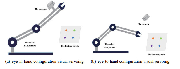
For constrained image-based visual servoing (IBVS) of robot manipulators, a model predictive control (MPC) strategy tuned by reinforcement learning (RL) is proposed in this study. First, model predictive control is used to transform the image-based visual servo task into a nonlinear optimization problem while taking system constraints into consideration. In the design of the model predictive controller, a depth-independent visual servo model is presented as the predictive model. Next, a suitable model predictive control objective function weight matrix is trained and obtained by a deep-deterministic-policy-gradient-based (DDPG) RL algorithm. Then, the proposed controller gives the sequential joint signals, so that the robot manipulator can respond to the desired state quickly. Finally, appropriate comparative simulation experiments are developed to illustrate the efficacy and stability of the suggested strategy.
- robot manipulator,
- image-based visual servoing,
- model predictive control,
- reinforcement learning
Citation: Jiashuai Li, Xiuyan Peng, Bing Li, Victor Sreeram, Jiawei Wu, Ziang Chen, Mingze Li. Model predictive control for constrained robot manipulator visual servoing tuned by reinforcement learning[J]. Mathematical Biosciences and Engineering, 2023, 20(6): 10495-10513. doi: 10.3934/mbe.2023463

Related Papers:

Abstract

For constrained image-based visual servoing (IBVS) of robot manipulators, a model predictive control (MPC) strategy tuned by reinforcement learning (RL) is proposed in this study. First, model predictive control is used to transform the image-based visual servo task into a nonlinear optimization problem while taking system constraints into consideration. In the design of the model predictive controller, a depth-independent visual servo model is presented as the predictive model. Next, a suitable model predictive control objective function weight matrix is trained and obtained by a deep-deterministic-policy-gradient-based (DDPG) RL algorithm. Then, the proposed controller gives the sequential joint signals, so that the robot manipulator can respond to the desired state quickly. Finally, appropriate comparative simulation experiments are developed to illustrate the efficacy and stability of the suggested strategy.

References

[1]	X. Liang, M. Peng, J. Lu, C. Qin, A visual servo control method for tomato cluster-picking manipulators based on a TS fuzzy neural network, Trans. ASABE, 64 (2021), 529–543. https://doi.org/10.13031/trans.13485 doi: 10.13031/trans.13485
[2]	R. J. Chang, C. Y. Lin, P. S. Lin, Visual-based automation of Peg-in-Hole microassembly process, Trans. ASABE, 133 (2011), 041015. https://doi.org/10.1115/1.4004497 doi: 10.1115/1.4004497
[3]	A. A. Palsdottir, M. Mohammadi, B. Bentsen, L. N. S. A. Struijk A dedicated tool frame based tongue interface layout improves 2D visual guided control of an assistive robotic manipulator: A design parameter for Tele-Applications, IEEE Sensors J., 22 (2022), 9868–9880. https://doi.org/10.1109/JSEN.2022.3164551 doi: 10.1109/JSEN.2022.3164551
[4]	Y. W. Zhang, Y. C. Liu, Z. W. Xie, Y. Liu, B. S. Cao, H. Liu, Visual servo control of the Macro/Micro manipulator with base vibration suppression and backlash compensation, App. Sci. Basel, 12 (2022). https://doi.org/10.3390/app12168386 doi: 10.3390/app12168386
[5]	R. Sharma, S. Shukla, L. Behera, Position-based visual servoing of a mobile robot with an automatic extrinsic calibration scheme, Robotica, 38 (2020), 831–844. https://doi.org/10.1017/S0263574719001115 doi: 10.1017/S0263574719001115
[6]	S. Heshmati-alamdari, A. Eqtami, G. C. Karras, D. V. Dimarogonas, K. J. Kyriakopoulos, A Self-triggered position based visual servoing model predictive control scheme for underwater robotic vehicles, Machines, 8 (2020). https://doi.org/10.3390/machines8020033 doi: 10.3390/machines8020033
[7]	Y. Zhao, W. F. Xie, S. Liu, Image-based visual servoing using improved image moments in 6-DOF robot systems, Int. J. Control Autom. Syst., 11 (2013), 586–596. https://doi.org/10.1007/s12555-012-0232-9 doi: 10.1007/s12555-012-0232-9
[8]	O. Tahri, H. Araujo, F. Chaumette, Y. Mezouar, Robust image-based visual servoing using invariant visual information, Robot. Auton. Syst., 61 (2013), 1588–1600. https://doi.org/10.1016/j.robot.2013.06.010 doi: 10.1016/j.robot.2013.06.010
[9]	D. J. Guo, X. Jin, D. Shao, J. Y. Li, Y. Shen, H. Tan, Image-based regulation of mobile robots without pose measurements, IEEE Control Syst. Lett., 6 (2022), 2156–2161. https://doi.org/10.1109/LCSYS.2021.3139288 doi: 10.1109/LCSYS.2021.3139288
[10]	N. Garcia-Aracil, C. Perez-Vidal, J. M. Sabater, R. Morales, F. J. Badesa, Robust and cooperative image-based visual servoing system using a redundant architecture, Sensors, 11 (2011), 11885–11900. https://doi.org/10.3390/s111211885 doi: 10.3390/s111211885
[11]	S. T. Liu, J. X. Dong, Robust online model predictive control for image-based visual servoing in polar coordinates, Trans. Inst. Meas. Control, 42 (2020), 890–903. https://doi.org/10.1177/0142331219895074 doi: 10.1177/0142331219895074
[12]	A. Rastegarpanah, A. Aflakian, R. Stolkin, Improving the manipulability of a redundant arm using decoupled hybrid visual servoing, Appl.Sci. Basel, 11 (2022). https://doi.org/10.3390/machines8020033 doi: 10.3390/machines8020033
[13]	Z. He, C. Wu, S. Zhang, X. Zhao, Moment-Based 2.5-D visual servoing for textureless planar part grasping, IEEE Trans. Ind. Electron., 66 (2019), 7821–7830. https://doi.org/10.1109/TIE.2018.2886783 doi: 10.1109/TIE.2018.2886783
[14]	F. Yan, B. Li, W. Shi, D. Wang, Hybrid visual servo trajectory tracking of wheeled mobile robots, IEEE Access, 6 (2018), 24291–24298. https://doi.org/10.1109/ACCESS.2018.2829839 doi: 10.1109/ACCESS.2018.2829839
[15]	X. J. Li, J. A. Gu, Z. D. Huang, C. Ji, S. X. Tang, Hierarchical multiloop MPC scheme for robot manipulators with nonlinear disturbance observer, Math. Biosci. Eng., 19 (2022), 12601–12616. https://doi.org/10.3934/mbe.2022588 doi: 10.3934/mbe.2022588
[16]	M. Mohammad Hossein Fallah, F. Janabi-Sharifi, Conjugated visual predictive control for constrained visual servoing, J. Intell. Robotic Syst., 101 (2021), 1–21. https://doi.org/10.1007/s10846-020-01299-6 doi: 10.1007/s10846-020-01299-6
[17]	Z. Qiu, S. Hu, X. Liang, Model predictive control for constrained image-based visual servoing in uncalibrated environments, Asian J. Control, 21 (2019), 783–799. https://doi.org/10.1002/asjc.1756 doi: 10.1002/asjc.1756
[18]	T. Wang, W. Xie, G. Liu, Y. Zhao, Quasi-min-max model predictive control for image-based visual servoing with tensor product model transformation, Asian J. Control, 17 (2015), 402–416. https://doi.org/10.1002/asjc.871 doi: 10.1002/asjc.871
[19]	J. Gao, G. Zhang, P. Wu, X. Zhao, T. Wang, W. Yan, Model predictive visual servoing of fully-actuated underwater vehicles with a sliding mode disturbance observer, IEEE Access, 7 (2019), 25516–25526. https://doi.org/10.1109/ACCESS.2019.2900998 doi: 10.1109/ACCESS.2019.2900998
[20]	Z. Jin, J. Wu, A. Liu, W. A. Zhang, L. Yu, Gaussian process-based nonlinear predictive control for visual servoing of constrained mobile robots with unknown dynamics, Robotics Auton. Syst., 136 (2021), 103712. https://doi.org/10.1016/j.robot.2020.103712 doi: 10.1016/j.robot.2020.103712
[21]	G. Allibert, E. Courtial, F. Chaumette, Predictive control for constrained image-based visual servoing, IEEE Trans. Robotics, 26 (2010), 933–939. https://doi.org/10.1109/TRO.2010.2056590 doi: 10.1109/TRO.2010.2056590
[22]	R. Shridhar, D. J. Cooper, A tuning strategy for unconstrained multivariable model predictive control, Indust. Eng. Chem. Res., 37 (1998), 4003–4016. https://doi.org/10.1021/ie980202s doi: 10.1021/ie980202s
[23]	R. Suzuki, F. Kawai, H. Ito, C. Nakazawa, Y. Fukuyama, E. Aiyoshi, Automatic tuning of model predictive control using particle swarm optimization, IEEE Swarm Intell. Symp., (2007), 221–226. https://doi.org/10.1109/SIS.2007.367941 doi: 10.1109/SIS.2007.367941
[24]	K. Han, J. Zhao, J. Qian, A novel robust tuning strategy for model predictive control, World Congr. Intell. Control Autom., 2 (2006), 6406–6410.
[25]	J. Van der Lee, W. Svrcek, B. Young, A tuning algorithm for model predictive controllers based on genetic algorithms and fuzzy decision making, ISA Trans., 47 (2008), 53–59. https://doi.org/10.1016/j.isatra.2007.06.003 doi: 10.1016/j.isatra.2007.06.003
[26]	S. Q. Chen, Y. Yang, R. Su, Deep reinforcement learning with emergent communication for coalitional negotiation games, Math. Biosci. Eng., 19 (2022), 4592–4609. https://doi.org/10.3934/mbe.2022212 doi: 10.3934/mbe.2022212
[27]	G. Ciaburro, Machine fault detection methods based on machine learning algorithms: A review, Math. Biosci. Eng., 19 (2021), 11453–11490. https://doi.org/10.3934/mbe.2022534 doi: 10.3934/mbe.2022534
[28]	M. Sedighizadeh, A. Rezazadeh, A modified adaptive wavelet PID control based on RL for wind energy conversion system control, Adv. Electr. Comput. Eng., 10 (2010), 153–159. https://doi.org/10.4316/AECE.2010.02027 doi: 10.4316/AECE.2010.02027
[29]	D. Lee, S. J. Lee, S. C. Yim, Reinforcement learning-based adaptive PID controller for DPS, Ocean Eng., 216 (2020), 108053. https://doi.org/10.1016/j.oceaneng.2020.108053 doi: 10.1016/j.oceaneng.2020.108053
[30]	I. Carlucho, M. De Paula, G. G. Acosta, Double Q-PID algorithm for mobile robot control, Expert Syst. Appl., 137 (2019), 292–307. https://doi.org/10.1016/j.eswa.2019.06.066 doi: 10.1016/j.eswa.2019.06.066
[31]	T. Chaffre, G. Le Chenadec, K. Sammut, E. Chauveau, B. Clement, Direct adaptive pole-placement controller using deep reinforcement learning: Application to auv control, IFAC-PapersOnLine, 54 (2021), 333–340. https://doi.org/10.1016/j.ifacol.2021.10.113 doi: 10.1016/j.ifacol.2021.10.113
[32]	M. Kang, H. Chen, J. X. Dong, Adaptive visual servoing with an uncalibrated camera using extreme learning machine and Q-leaning, Neurocomputing, 402 (2020), 384–394. https://doi.org/10.1016/j.neucom.2020.03.049 doi: 10.1016/j.neucom.2020.03.049
[33]	M. Mehndiratta, E. Camci, E. Kayacan, Automated tuning of nonlinear model predictive controller by reinforcement learning, IEEE/RSJ Int. Confer. Intell. Robots Syst., (2018), 3016–3021.
[34]	P. T. Jardine, S. N. Givigi, S. Yousefi, Experimental results for autonomous model-predictive trajectory planning tuned with machine learning, IEEE Int. Syst. Confer., (2017), 663–669.
[35]	K. M. Cabral, S. R. B. dos Santos, S. N. Givigi, C. L. Nascimento, Design of model predictive control via learning automata for a single UAV load transportation, IEEE Int. Syst. Confer., (2017), 656–662.
[36]	F. Wang, B. M. Ren, Y. Liu, B. Cui, Tracking moving target for 6 degree-of-freedom robot manipulator with adaptive visual servoing based on deep reinforcement learning PID controller, Rev. Sci. Instrum., 93 (2022), 045108. https://doi.org/10.1063/5.0087561 doi: 10.1063/5.0087561
[37]	Z. H. Jin, J. H. Wu, A. D. Liu, W. A. Zhang, L. Yu, Policy-based deep reinforcement learning for visual servoing control of mobile robots With visibility constraints, IEEE Trans. Ind. Electron., 69 (2021), 1898–1908. https://doi.org/10.1109/TIE.2021.3057005 doi: 10.1109/TIE.2021.3057005
[38]	Y. C. Liu, C. Y. Huang, DDPG-based adaptive robust tracking control for aerial manipulators with decoupling approach, IEEE Trans. Cybern., 52 (2021), 8258–8271. https://doi.org/10.1109/TIE.2021.3057005 doi: 10.1109/TIE.2021.3057005
[39]	P. M. Kebria, S. Al-Wais, H. Abdi, S. Nahavandi, Kinematic and dynamic modelling of ur5 manipulator, IEEE Int. Confer. Syst. Man Cybern., (2016), 004229–004234.
[40]	F. Chaumette, S. Hutchinson, Visual servo control. i. basic approaches, IEEE Robotics Autom. Mag., 13 (2006), 82–90. https://doi.org/10.1109/MRA.2006.250573 doi: 10.1109/MRA.2006.250573

Reader Comments

Your name:*

Email:*
© 2023 the Author(s), licensee AIMS Press. This is an open access article distributed under the terms of the Creative Commons Attribution License (http://creativecommons.org/licenses/by/4.0)