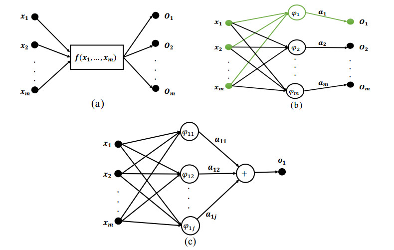
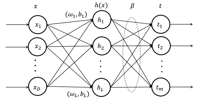
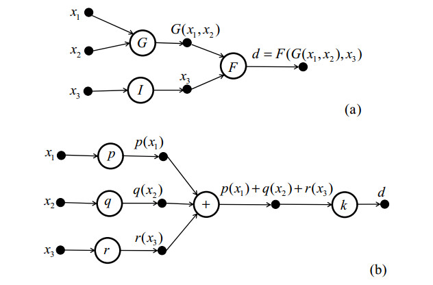
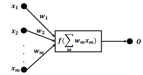
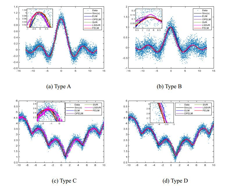
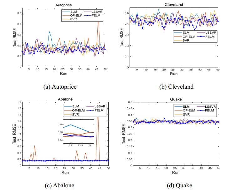
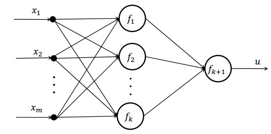
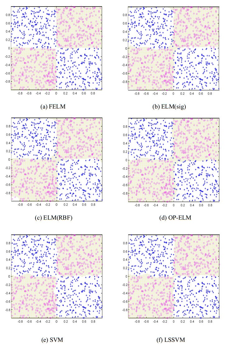
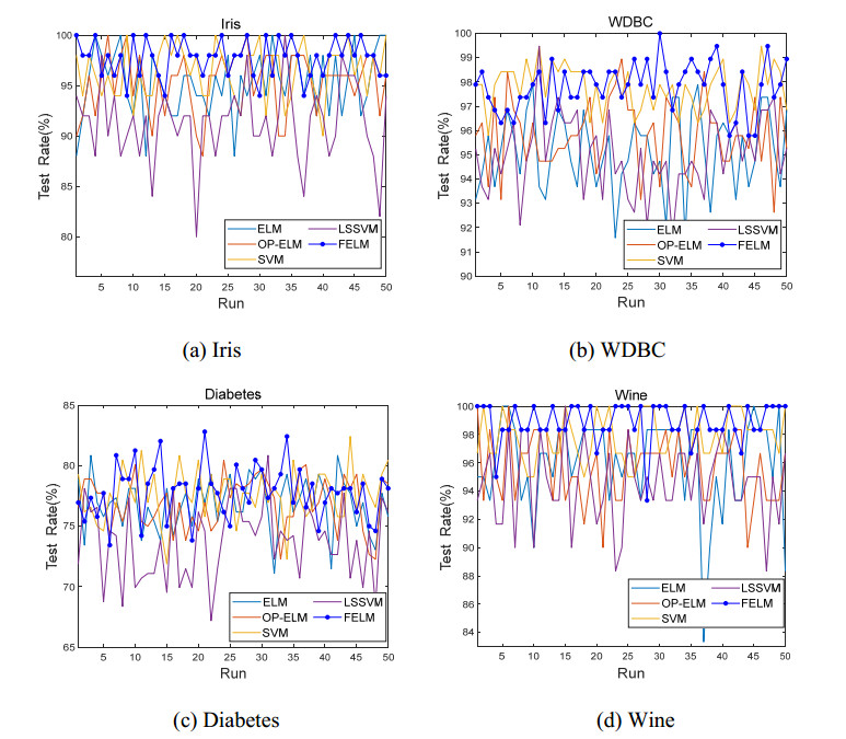
Although Extreme Learning Machine (ELM) can learn thousands of times faster than traditional slow gradient algorithms for training neural networks, ELM fitting accuracy is limited. This paper develops Functional Extreme Learning Machine (FELM), which is a novel regression and classifier. It takes functional neurons as the basic computing units and uses functional equation-solving theory to guide the modeling process of functional extreme learning machines. The functional neuron function of FELM is not fixed, and its learning process refers to the process of estimating or adjusting the coefficients. It follows the spirit of extreme learning and solves the generalized inverse of the hidden layer neuron output matrix through the principle of minimum error, without iterating to obtain the optimal hidden layer coefficients. To verify the performance of the proposed FELM, it is compared with ELM, OP-ELM, SVM and LSSVM on several synthetic datasets, XOR problem, benchmark regression and classification datasets. The experimental results show that although the proposed FELM has the same learning speed as ELM, its generalization performance and stability are better than ELM.
Citation: Xianli Liu, Yongquan Zhou, Weiping Meng, Qifang Luo. Functional extreme learning machine for regression and classification[J]. Mathematical Biosciences and Engineering, 2023, 20(2): 3768-3792. doi: 10.3934/mbe.2023177
Although Extreme Learning Machine (ELM) can learn thousands of times faster than traditional slow gradient algorithms for training neural networks, ELM fitting accuracy is limited. This paper develops Functional Extreme Learning Machine (FELM), which is a novel regression and classifier. It takes functional neurons as the basic computing units and uses functional equation-solving theory to guide the modeling process of functional extreme learning machines. The functional neuron function of FELM is not fixed, and its learning process refers to the process of estimating or adjusting the coefficients. It follows the spirit of extreme learning and solves the generalized inverse of the hidden layer neuron output matrix through the principle of minimum error, without iterating to obtain the optimal hidden layer coefficients. To verify the performance of the proposed FELM, it is compared with ELM, OP-ELM, SVM and LSSVM on several synthetic datasets, XOR problem, benchmark regression and classification datasets. The experimental results show that although the proposed FELM has the same learning speed as ELM, its generalization performance and stability are better than ELM.

| [1] | L. C. Jiao, S. Y. Yang, F. Liu, S. G. Wang, Z. X. Feng, Seventy years beyond neural networks: retrospect and prospect, Chin. J. Comput., 39 (2016), 1697–1716. |
| [2] |
O. I. Abiodun, A. Jantan, A. E. Omolara, K. V. Dada, N. A. Mohamed, H. Arshad, State-of-the-art in artificial neural network applications: A survey, Heliyon, 4 (2018), e00938. https://doi.org/10.1016/j.heliyon.2018.e00938 doi: 10.1016/j.heliyon.2018.e00938

|
| [3] |
A. K. Jain, J. Mao, K. M. Mohiuddin, Artificial neural networks: A tutorial, Computer, 29 (1996), 31–44. https://doi.org/10.1109/2.485891 doi: 10.1109/2.485891
|
| [4] | P. Werbos, Beyond Regression: New Tools for Prediction and Analysis in the Behavioral Sciences, Ph.D thesis, Harvard University, Boston, USA, 1974. |
| [5] | D. E. Rumelhart, J. L. McClelland, Parallel Distributed Processing: Explorations in the Microstructure of Cognition, MIT Press, Cambridge, USA, 1986. https://doi.org/10.7551/mitpress/5236.001.0001 |
| [6] | K. Vora, S. Yagnik, M. Scholar, A survey on backpropagation algorithms for feedforward neural networks, Int. J. Eng. Dev. Res., 1 (2014), 193–197. |
| [7] |
S. Ding, C. Su, J. Yu, An optimizing BP neural network algorithm based on genetic algorithm, Artif. Intell. Rev., 36 (2011), 153–162. https://doi.org/10.1007/s10462-011-9208-z doi: 10.1007/s10462-011-9208-z
|
| [8] |
A. Sapkal, U. V. Kulkarni, Modified backpropagation with added white Gaussian noise in weighted sum for convergence improvement, Procedia Comput. Sci., 143 (2018), 309–316. https://doi.org/10.1016/j.procs.2018.10.401 doi: 10.1016/j.procs.2018.10.401
|
| [9] |
W. Yang, X. Liu, K. Wang, J. Hu, G. Geng, J. Feng, Sex determination of three-dimensional skull based on improved backpropagation neural network, Comput. Math. Methods Med., 2019 (2019), 1–8. https://doi.org/10.1155/2019/9163547 doi: 10.1155/2019/9163547
|
| [10] |
W. C. Pan, S. D. Liu, Optimization research and application of BP neural network, Comput. Technol. Dev., 29 (2019), 74–76. https://doi.org/10.3969/j.issn.1673-629X.2019.05.016 doi: 10.3969/j.issn.1673-629X.2019.05.016
|
| [11] |
G. B. Huang, Q. Y. Zhu, C. K. Siew, Extreme learning machine: theory and applications, Neurocomputing, 70 (2006), 489–501. https://doi.org/10.1016/j.neucom.2005.12.126 doi: 10.1016/j.neucom.2005.12.126
|
| [12] |
S. Y. Lu, Z. H. Lu, S. H. Wang, Y. D. Zhang, Review of extreme learning machine, Meas. Control Technol., 37 (2018), 3–9. https://doi.org/10.19708/j.ckjs.2018.10.001 doi: 10.19708/j.ckjs.2018.10.001
|
| [13] |
F. Mohanty, S. Rup, B. Dash, B. Majhi, M. N. S. Swamy, A computer-aided diagnosis system using Tchebichef features and improved grey wolf optimized extreme learning machine, Appl. Intell., 49 (2019), 983–1001. https://doi.org/10.1007/s10489-018-1294-z doi: 10.1007/s10489-018-1294-z
|
| [14] |
D. Muduli, R. Dash, B. Majhi, Automated breast cancer detection in digital mammograms: A moth flame optimization based ELM approach, Biomed. Signal Process. Control, 59 (2020), 101912. https://doi.org/10.1016/j.bspc.2020.101912 doi: 10.1016/j.bspc.2020.101912
|
| [15] |
Z. Wang, Y. Luo, J. Xin, H. Zhang, L. Qu, Z. Wang, et al., Computer-aided diagnosis based on extreme learning machine: a review, IEEE Access, 8 (2020), 141657–141673. https://doi.org/10.1109/ACCESS.2020.3012093 doi: 10.1109/ACCESS.2020.3012093
|
| [16] |
Z. Huang, Y. Yu, J. Gu, H. Liu, An efficient method for traffic sign recognition based on extreme learning machine, IEEE Trans. Cybern., 47 (2016), 920–933. https://doi.org/10.1109/TCYB.2016.2533424 doi: 10.1109/TCYB.2016.2533424
|
| [17] |
S. Aziz, E. A. Mohamed, F. Youssef, Traffic sign recognition based on multi-feature fusion and ELM classifier, Procedia Comput. Sci., 127 (2018), 146–153. https://doi.org/10.1016/j.procs.2018.01.109 doi: 10.1016/j.procs.2018.01.109
|
| [18] |
Z. M. Yaseen, S. O. Sulaiman, R. C. Deo, K. W. Chau, An enhanced extreme learning machine model for river flow forecasting: State-of-the-art, practical applications in water resource engineering area and future research direction, J. Hydrol., 569 (2019), 387–408. https://doi.org/10.1016/j.jhydrol.2018.11.069 doi: 10.1016/j.jhydrol.2018.11.069
|
| [19] |
M. Shariati, M. S. Mafipour, B. Ghahremani, F. Azarhomayun, M. Ahmadi, M. T. Trung, et al., A novel hybrid extreme learning machine-grey wolf optimizer (ELM-GWO) model to predict compressive strength of concrete with partial replacements for cement, Eng. Comput., 38 (2020), 757–779. https://doi.org/10.1007/s00366-020-01081-0 doi: 10.1007/s00366-020-01081-0
|
| [20] |
R. Xu, X. Liang, J. S. Qi, Z. Y. Li, S. S. Zhang, Advances and trends in extreme learning machine, Chin. J. Comput., 42 (2019), 1640–1670. https://doi.org/10.11897/SP.J.1016.2019.01640 doi: 10.11897/SP.J.1016.2019.01640
|
| [21] |
J. Wang, S. Lu, S. H. Wang, Y. D. Zhang, A review on extreme learning machine, Multimedia Tools Appl., 81 (2022), 41611–41660. https://doi.org/10.1007/s11042-021-11007-7 doi: 10.1007/s11042-021-11007-7
|
| [22] | W. Deng, Q. Zheng, L. Chen, Regularized extreme learning machine, in 2009 IEEE Symposium on Computational Intelligence and Data Mining, IEEE, Nashville, USA, (2009), 389–395. https://doi.org/10.1109/CIDM.2009.4938676 |
| [23] |
Y. P. Zhao, Q. K. Hu, J. G. Xu, B. Li, G. Huang, Y. T. Pan, A robust extreme learning machine for modeling a small-scale turbojet engine, Appl. Energy, 218 (2018), 22–35. https://doi.org/10.1016/j.apenergy.2018.02.175 doi: 10.1016/j.apenergy.2018.02.175
|
| [24] |
K. Wang, H. Pei, J. Cao, P. Zhong, Robust regularized extreme learning machine for regression with non-convex loss function via DC program, J. Franklin Inst., 357 (2020), 7069–7091. https://doi.org/10.1016/j.jfranklin.2020.05.027 doi: 10.1016/j.jfranklin.2020.05.027
|
| [25] |
X. Lu, L. Ming, W. Liu, H. X. Li, Probabilistic regularized extreme learning machine for robust modeling of noise data, IEEE Trans. Cybern., 48 (2018), 2368–2377. https://doi.org/10.1109/TCYB.2017.2738060 doi: 10.1109/TCYB.2017.2738060
|
| [26] |
H. Yıldırım, M. Revan Özkale, LL-ELM: A regularized extreme learning machine based on L1-norm and Liu estimator, Neural Comput. Appl., 33 (2021), 10469–10484. https://doi.org/10.1007/s00521-021-05806-0 doi: 10.1007/s00521-021-05806-0
|
| [27] |
G. B. Huang, H. Zhou, X. Ding, R. Zhang, Extreme learning machine for regression and multiclass classification, IEEE Trans. Syst. Man Cybern. Part B Cybern., 42 (2012), 513–529. https://doi.org/10.1109/TSMCB.2011.2168604 doi: 10.1109/TSMCB.2011.2168604
|
| [28] |
X. Liu, L. Wang, G. B. Huang, J. Zhang, J. Yin, Multiple kernel extreme learning machine, Neurocomputing, 149 (2015), 253–264. https://doi.org/10.1016/j.neucom.2013.09.072 doi: 10.1016/j.neucom.2013.09.072
|
| [29] |
N. Y. Liang, G. B. Huang, P. Saratchandran, N. Sundararajan, A fast and accurate online sequential learning algorithm for feedforward networks, IEEE Trans. Neural Networks, 17 (2006), 1411–1423. https://doi.org/10.1109/TNN.2006.880583 doi: 10.1109/TNN.2006.880583
|
| [30] |
J. Yang, F. Ye, H. J. Rong, B. Chen, Recursive least mean p-power extreme learning machine, Neural Networks, 91 (2017), 22–33. https://doi.org/10.1016/j.neunet.2017.04.001 doi: 10.1016/j.neunet.2017.04.001
|
| [31] |
J. Yang, Y. Xu, H. J. Rong, S. Du, B. Chen, Sparse recursive least mean p-power extreme learning machine for regression, IEEE Access, 6 (2018), 16022–16034. https://doi.org/10.1109/ACCESS.2018.2815503 doi: 10.1109/ACCESS.2018.2815503
|
| [32] |
S. Ding, B. Mirza, Z. Lin, J. Cao, X. Lai, T. V. Nguyen, et al., Kernel based online learning for imbalance multiclass classification, Neurocomputing, 277 (2018), 139–148. https://doi.org/10.1016/j.neucom.2017.02.102 doi: 10.1016/j.neucom.2017.02.102
|
| [33] |
S. Shukla, B. S. Raghuwanshi, Online sequential class-specific extreme learning machine for binary imbalanced learning, Neural Networks, 119 (2019), 235–248. https://doi.org/10.1016/j.neunet.2019.08.018 doi: 10.1016/j.neunet.2019.08.018
|
| [34] |
F. Lu, J. Wu, J. Huang, X. Qiu, Aircraft engine degradation prognostics based on logistic regression and novel OS-ELM algorithm, Aerosp. Sci. Technol., 84 (2019), 661–671. https://doi.org/10.1016/j.ast.2018.09.044 doi: 10.1016/j.ast.2018.09.044
|
| [35] |
H. Yu, H. Xie, X. Yang, H. Zou, S. Gao, Online sequential extreme learning machine with the increased classes, Comput. Electr. Eng., 90 (2021), 107008. https://doi.org/10.1016/j.compeleceng.2021.107008 doi: 10.1016/j.compeleceng.2021.107008
|
| [36] |
Q. Y. Zhu, A. K. Qin, P. N. Suganthan, G. B. Huang, Evolutionary extreme learning machine, Pattern Recognit., 38 (2005), 1759–1763. https://doi.org/10.1016/j.patcog.2005.03.028 doi: 10.1016/j.patcog.2005.03.028
|
| [37] |
D. T. Bui, P. T. T. Ngo, T. D. Pham, A. Jaafari, N. Q. Minh, P. V. Hoa, et al., A novel hybrid approach based on a swarm intelligence optimized extreme learning machine for flash flood susceptibility mapping, Catena, 179 (2019), 184–196. https://doi.org/10.1016/j.catena.2019.04.009 doi: 10.1016/j.catena.2019.04.009
|
| [38] |
W. Cai, J. Yang, Y. Yu, Y. Song, T. Zhou, J. Qin, PSO-ELM: A hybrid learning model for short-term traffic flow forecasting, IEEE Access, 8 (2020), 6505–6514. https://doi.org/10.1109/ACCESS.2019.2963784 doi: 10.1109/ACCESS.2019.2963784
|
| [39] |
J. Zeng, B. Roy, D. Kumar, A. S. Mohammed, D. J. Armaghani, J. Zhou, et al., Proposing several hybrid PSO-extreme learning machine techniques to predict TBM performance, Eng. Comput., 38 (2022), 3811–3827. https://doi.org/10.1007/s00366-020-01225-2 doi: 10.1007/s00366-020-01225-2
|
| [40] |
R. M. Adnan, R. R. Mostafa, O. Kisi, Z. M. Yaseen, S. Shahid, M. Zounemat-Kermani, Improving streamflow prediction using a new hybrid ELM model combined with hybrid particle swarm optimization and grey wolf optimization, Knowl.-Based Syst., 230 (2021), 107379. https://doi.org/10.1016/j.knosys.2021.107379 doi: 10.1016/j.knosys.2021.107379
|
| [41] |
G. B. Huang, L. Chen, C. K. Siew, Universal approximation using incremental constructive feedforward networks with random hidden nodes, IEEE Trans. Neural Networks, 17 (2006), 879–892. https://doi.org/10.1109/tnn.2006.875977 doi: 10.1109/tnn.2006.875977
|
| [42] |
G. B. Huang, M. B. Li, L. Chen, C. K. Siew, Incremental extreme learning machine with fully complex hidden nodes, Neurocomputing, 71 (2008), 576–583. https://doi.org/10.1016/j.neucom.2007.07.025 doi: 10.1016/j.neucom.2007.07.025
|
| [43] |
Y. X. Wu, D. Liu, H. Jiang, Length-changeable incremental extreme learning machine, J. Comput. Sci. Technol., 32 (2017), 630–643. https://doi.org/10.1007/s11390-017-1746-7 doi: 10.1007/s11390-017-1746-7
|
| [44] |
S. Song, M. Wang, Y. Lin, An improved algorithm for incremental extreme learning machine, Syst. Sci. Control Eng., 8 (2020), 308–317. https://doi.org/10.1080/21642583.2020.1759156 doi: 10.1080/21642583.2020.1759156
|
| [45] |
H. C. Leung, C. S. Leung, E. W. M. Wong, Fault and noise tolerance in the incremental extreme learning machine, IEEE Access, 7 (2019), 155171–155183. https://doi.org/10.1109/ACCESS.2019.2948059 doi: 10.1109/ACCESS.2019.2948059
|
| [46] |
H. J. Rong, Y. S. Ong, A. H. Tan, Z. Zhu, A fast pruned-extreme learning machine for classification problem, Neurocomputing, 72 (2008), 359–366. https://doi.org/10.1016/j.neucom.2008.01.005 doi: 10.1016/j.neucom.2008.01.005
|
| [47] |
Y. Miche, A. Sorjamaa, P. Bas, O. Simula, C. Jutten, A. Lendasse, OP-ELM: optimally pruned extreme learning machine, IEEE Trans. Neural Networks, 21 (2010), 158–162. https://doi.org/10.1109/TNN.2009.2036259 doi: 10.1109/TNN.2009.2036259
|
| [48] |
R. M. Adnan, Z. Liang, S. Trajkovic, M. Zounemat-Kermani, B. Li, O. Kisi, Daily streamflow prediction using optimally pruned extreme learning machine, J. Hydrol., 577 (2019), 123981. https://doi.org/10.1016/j.jhydrol.2019.123981 doi: 10.1016/j.jhydrol.2019.123981
|
| [49] |
Q. Fan, L. Niu, Q. Kang, Q. Kang, Regression and multiclass classification using sparse extreme learning machine via smoothing group L1/2 regularizer, IEEE Access, 8 (2020), 191482–191494. https://doi.org/10.1109/ACCESS.2020.3031647 doi: 10.1109/ACCESS.2020.3031647
|
| [50] |
B. Li, Y. P. Zhao, Group reduced kernel extreme learning machine for fault diagnosis of aircraft engine, Eng. Appl. Artif. Intell., 96 (2020), 103968. https://doi.org/10.1016/j.engappai.2020.103968 doi: 10.1016/j.engappai.2020.103968
|
| [51] |
G. Feng, Y. Lan, X. Zhang, Z. Qian, Dynamic adjustment of hidden node parameters for extreme learning machine, IEEE Trans. Cybern., 45 (2015), 279–288. https://doi.org/10.1109/TCYB.2014.2325594 doi: 10.1109/TCYB.2014.2325594
|
| [52] |
G. Zeng, B. Zhang, F. Yao, S. Chai, Modified bidirectional extreme learning machine with Gram-Schmidt orthogonalization method, Neurocomputing, 316 (2018), 405–414. https://doi.org/10.1016/j.neucom.2018.08.029 doi: 10.1016/j.neucom.2018.08.029
|
| [53] |
M. Pratama, G. Zhang, M. J. Er, S. Anavatti, An incremental type-2 meta-cognitive extreme learning machine, IEEE Trans. Cybern., 47 (2017), 339–353. https://doi.org/10.1109/TCYB.2016.2514537 doi: 10.1109/TCYB.2016.2514537
|
| [54] |
Z. Chen, C. Jiang, L. Xie, A novel ensemble ELM for human activity recognition using smartphone sensors, IEEE Trans. Ind. Inf., 15 (2019), 2691–2699. https://doi.org/10.1109/TⅡ.2018.2869843 doi: 10.1109/TⅡ.2018.2869843
|
| [55] |
S. F. Stefenon, R. B. Grebogi, R. Z. Freire, A. Nied, L. H. Meyer, Optimized ensemble extreme learning machine for classification of electrical insulators conditions, IEEE Trans. Ind. Electron., 67 (2020), 5170–5178. https://doi.org/10.1109/TIE.2019.2926044 doi: 10.1109/TIE.2019.2926044
|
| [56] |
X. B. Wang, X. Zhang, Z. Li, J. Wu, Ensemble extreme learning machines for compound-fault diagnosis of rotating machinery, Knowl.-Based Syst., 188 (2020), 105012. https://doi.org/10.1016/j.knosys.2019.105012 doi: 10.1016/j.knosys.2019.105012
|
| [57] |
X. Zhou, Y. Zhang, Ensemble extreme learning machine approach to thermal infrared subpixel temperature estimation, IEEE Geosci. Remote Sens. Lett., 18 (2021), 920–924. https://doi.org/10.1109/LGRS.2020.2985500 doi: 10.1109/LGRS.2020.2985500
|
| [58] |
D. Lam, D. Wunsch, Unsupervised feature learning classification with radial basis function extreme learning machine using graphic processors, IEEE Trans. Cybern., 47 (2017), 224–231. https://doi.org/10.1109/TCYB.2015.2511149 doi: 10.1109/TCYB.2015.2511149
|
| [59] |
L. Yao, Z. Ge, Distributed parallel deep learning of hierarchical extreme learning machine for multimode quality prediction with big process data, Eng. Appl. Artif. Intell., 81 (2019), 450–465. https://doi.org/10.1016/j.engappai.2019.03.011 doi: 10.1016/j.engappai.2019.03.011
|
| [60] |
M. Duan, K. Li, X. Liao, K. Li, A parallel multiclassification algorithm for big data using an extreme learning machine, IEEE Trans. Neural Networks Learn. Syst., 29 (2018), 2337–2351. https://doi.org/10.1109/TNNLS.2017.2654357 doi: 10.1109/TNNLS.2017.2654357
|
| [61] |
J. Tang, C. Deng, G. B. Huang, Extreme learning machine for multilayer perceptron, IEEE Trans. Neural Networks Learn. Syst., 27 (2016), 809–821. https://doi.org/10.1109/TNNLS.2015.2424995 doi: 10.1109/TNNLS.2015.2424995
|
| [62] |
C. M. Wong, C. M. Vong, P. K. Wong, J. Cao, Kernel-based multilayer extreme learning machines for representation learning, IEEE Trans. Neural Networks Learn. Syst., 29 (2018), 757–762. https://doi.org/10.1109/TNNLS.2016.2636834 doi: 10.1109/TNNLS.2016.2636834
|
| [63] |
H. Dai, J. Cao, T. Wang, M. Deng, Z. Yang, Multilayer one-class extreme learning machine, Neural Networks, 115 (2019), 11–22. https://doi.org/10.1016/j.neunet.2019.03.004 doi: 10.1016/j.neunet.2019.03.004
|
| [64] |
J. Zhang, Y. Li, W. Xiao, Z. Zhang, Non-iterative and fast deep learning: Multilayer extreme learning machines, J. Franklin Inst., 357 (2020), 8925–8955. https://doi.org/10.1016/j.jfranklin.2020.04.033 doi: 10.1016/j.jfranklin.2020.04.033
|
| [65] |
S. Yahia, S. Said, M. Zaied, Wavelet extreme learning machine and deep learning for data classification, Neurocomputing, 470 (2022), 280–289. https://doi.org/10.1016/j.neucom.2020.04.158 doi: 10.1016/j.neucom.2020.04.158
|
| [66] |
E. Castillo, Functional networks, Neural Process. Lett., 7 (1998), 151–159. https://doi.org/10.1023/A:1009656525752 doi: 10.1023/A:1009656525752
|
| [67] |
Y. Q. Zhou, L. C. Jiao, Universal learning algorithm of hierarchical function networks, Chin. J. Comput., 28 (2005), 1277–1286. https://doi.org/10.3321/j.issn:0254-4164.2005.08.004 doi: 10.3321/j.issn:0254-4164.2005.08.004
|
| [68] | Y. Q. Zhou, B. Zhao, L. C. Jiao, Serial function networks method and learning algorithm with applications, Chin. J. Comput., 31 (2008), 1073–1081. |
| [69] |
G. Zhou, Y. Zhou, H. Huang, Z. Tang, Functional networks and applications: A survey, Neurocomputing, 335 (2019), 384–399. https://doi.org/10.1016/j.neucom.2018.04.085 doi: 10.1016/j.neucom.2018.04.085
|
| [70] | A. Asuncion, D. J. Newman, UCI machine learning repository, School of Information and Computer Science, University of California, Irvine, CA, 2007. Available from: http://www.ics.uci.edu/~mlearn/MLRepository.html. |
| [71] | StatLib DataSets Archive. Available from: http://lib.stat.cmu.edu/datasets. |
Figures(9) / Tables(14)

Xianli Liu, Yongquan Zhou, Weiping Meng, Qifang Luo. Functional extreme learning machine for regression and classification[J]. Mathematical Biosciences and Engineering, 2023, 20(2): 3768-3792. doi: 10.3934/mbe.2023177


 DownLoad: