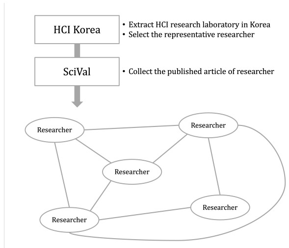
Since information and communication technology (ICT) has become one of the leading and essential fields for allowing developing countries to have the major growth engines, the majority of the countries have promoted collaboration in every ICT-related topics. In this study, we performed the trend and collaboration network analysis (CNA) in Korea for 2010–2019 among researchers who are related to human–computer interaction, one of the hottest research areas in ICT. Publication data were collected from SciVal, and the collaboration network was determined using degree, closeness, betweenness centralities, and PageRank. Hence, key researchers were identified based on their centrality metrics. The dataset contained 7,155 publications, thus reflecting the contributions of a total of 243 authors. The results of our data analysis demonstrated that key researchers can be identified via CNA; this aspect was not evident from the results of the most productive researchers. Additionally, on the basis of the results, the implications and limitations of this study were analyzed.
Citation: Seungpeel Lee, Jisu Kim, Eun Been Choi, Sojung Shin, Dogun Kim, HyeRim Yu, Seoyun Kim, Wongi S. Na, Eunil Park. Computational analysis of a collaboration network on human-computer interaction in Korea[J]. Mathematical Biosciences and Engineering, 2022, 19(12): 13911-13927. doi: 10.3934/mbe.2022648
Since information and communication technology (ICT) has become one of the leading and essential fields for allowing developing countries to have the major growth engines, the majority of the countries have promoted collaboration in every ICT-related topics. In this study, we performed the trend and collaboration network analysis (CNA) in Korea for 2010–2019 among researchers who are related to human–computer interaction, one of the hottest research areas in ICT. Publication data were collected from SciVal, and the collaboration network was determined using degree, closeness, betweenness centralities, and PageRank. Hence, key researchers were identified based on their centrality metrics. The dataset contained 7,155 publications, thus reflecting the contributions of a total of 243 authors. The results of our data analysis demonstrated that key researchers can be identified via CNA; this aspect was not evident from the results of the most productive researchers. Additionally, on the basis of the results, the implications and limitations of this study were analyzed.

| [1] | K. Hornbæk, A. Oulasvirta, S. Reeves, S. Bødker, What to study in hci?, in Proc. of CHI EA '15, (2015), 2385–2388. https://doi.org/10.1145/2702613.2702648 |
| [2] | A. Abdul, J. Vermeulen, D. Wang, B. Lim, M. Kankanhalli, Trends and trajectories for explainable, accountable and intelligible systems: An hci research agenda, in Proc. of CHI '18, (2018), 1–18. https://doi.org/10.1145/3173574.3174156 |
| [3] | J. Huang, Z. Zhuang, J. Li, C. L. Giles, Collaboration over time: Characterizing and modeling network evolution, in Proc. of WSDM '08, (2008), 107–116. https://doi.org/10.1145/1341531.1341548 |
| [4] |
F. Cheng, Y. Huang, D. Tsaih, C. Wu, Trend analysis of co-authorship network in library hi tech, Library Hi Tech., 37 (2019), 43–56. https://doi.org/10.1108/LHT-11-2017-0241 doi: 10.1108/LHT-11-2017-0241

|
| [5] |
B. Fida, F. Cutolo, G. di Franco, M. Ferrari, V. Ferrari, Augmented reality in open surgery, Updates Surgery, 70 (2018), 389–400. https://doi.org/10.1007/s13304-018-0567-8 doi: 10.1007/s13304-018-0567-8
|
| [6] |
S. D. J. Barbosa, M. S. Silveira, I. Gasparini, What publications metadata tell us about the evolution of a scientific community: The case of the brazilian human–computer interaction conference series, Scientometrics, 110 (2017), 275–300. https://doi.org/10.1007/s11192-016-2162-4 doi: 10.1007/s11192-016-2162-4
|
| [7] |
S. Uddin, L. Hossain, A. Abbasi, K. Rasmussen, Trend and efficiency analysis of co-authorship network, Scientometrics, 90 (2012), 687–699. https://doi.org/10.1007/s11192-011-0511-x doi: 10.1007/s11192-011-0511-x
|
| [8] |
J. Larrosa, Co-authorship networks of argentine economists, J. Econom. Finance Administr. Sci., 24 (2019), 82–96. https://doi.org/10.1108/JEFAS-06-2018-0062 doi: 10.1108/JEFAS-06-2018-0062
|
| [9] |
K. Lee, T. Nam, Hci in korea: Where imagination becomes reality, Interactions, 22 (2015), 48–51. https://doi.org/10.1145/2688446 doi: 10.1145/2688446
|
| [10] |
J. Y. Lee, M. Kam, N. G. Han, H. Song, Analysis of the role of library and information science related research efforts in korean human computer interaction subject field, J. Korean Soc. Inform. Manag., 33 (2016), 177–200. https://doi.org/10.3743/KOSIM.2016.33.2.177 doi: 10.3743/KOSIM.2016.33.2.177
|
| [11] | T. T. Hewett, R. Baecker, S. Card, T. Carey, J. Gasen, M. Mantei, et al., ACM SIGCHI curricula for human-computer interaction, ACM, 1992. https://doi.org/10.1145/2594128 |
| [12] | R. W. Pew, Evolution of human-computer interaction: from memex to bluetooth and beyond, in The human-computer interaction handbook: Fundamentals, evolving technologies and emerging applications, CRC Press, (2002), 1–17. |
| [13] | H. Lee, J. H. Park, Y. Song, Research collaboration networks of prolific institutions in the hci field in korea: An analysis of the hci korea conference proceedings, in Proceedings of HCI Korea '14, The HCI Society of Korea, (2014), 434–441. |
| [14] | K. Lee, J. Lee, Usability in korea–from gui to user experience design, in Global usability, Springer, (2011), 309–331. https://doi.org/10.1007/978-0-85729-304-6_19 |
| [15] |
L. Kang, S. Jackson, Collaborative art practice as hci research, Interactions, 25 (2018), 78–81. https://doi.org/10.1145/3177816 doi: 10.1145/3177816
|
| [16] |
S. Lee, B. Bozeman, The impact of research collaboration on scientific productivity, Soc. Studies Sci., 35 (2005), 673–702. https://doi.org/10.1177/0306312705052359 doi: 10.1177/0306312705052359
|
| [17] |
A. Higaki, T. Uetani, S. Ikeda, O. Yamaguchi, Co-authorship network analysis in cardiovascular research utilizing machine learning (2009–2019), Int. J. Med. Inform., 143 (2020), 104274. https://doi.org/10.1016/j.ijmedinf.2020.104274 doi: 10.1016/j.ijmedinf.2020.104274
|
| [18] |
F. Parand, H. Rahimi, M. Gorzin, Combining fuzzy logic and eigenvector centrality measure in social network analysis, Phys. A Statist. Mechan. Appl., 459 (2016), 24–31. https://doi.org/10.1016/j.physa.2016.03.079 doi: 10.1016/j.physa.2016.03.079
|
| [19] |
J. M. Bolland, Sorting out centrality: An analysis of the performance of four centrality models in real and simulated networks, Social Networks, 10 (1988), 233–253. https://doi.org/10.1016/0378-8733(88)90014-7 doi: 10.1016/0378-8733(88)90014-7
|
| [20] |
A. Bavelas, A mathematical model for group structures, Appl. Anthropol., 7 (1948), 16–30. https://doi.org/10.17730/humo.7.3.f4033344851gl053 doi: 10.17730/humo.7.3.f4033344851gl053
|
| [21] |
E. Yan, Y, Ding, Applying centrality measures to impact analysis: A coauthorship network analysis, J. Am. Soc. Inform. Sci. Technol., 60 (2009), 2107–2118. https://doi.org/10.1002/asi.21128 doi: 10.1002/asi.21128
|
| [22] |
F. J. Acedo, C. Barroso, C. Casanueva, J. Galán, Co-authorship in management and organizational studies: An empirical and network analysis, J. Manag. Studies, 43 (2006), 957–983. https://doi.org/10.1111/j.1467-6486.2006.00625.x doi: 10.1111/j.1467-6486.2006.00625.x
|
| [23] |
L. Yin, H. Kretschmer, R. A. Hanneman, Z. Liu, Connection and stratification in research collaboration: An analysis of the collnet network, Inform. Process. Manag., 42 (2006), 1599–1613. https://doi.org/10.1016/j.ipm.2006.03.021 doi: 10.1016/j.ipm.2006.03.021
|
| [24] |
S. Brin, L. Page, The anatomy of a large-scale hypertextual web search engine, Comput. Networks ISDN Syst., 30 (1998), 107–117. https://doi.org/10.1016/S0169-7552(98)00110-X doi: 10.1016/S0169-7552(98)00110-X
|
| [25] | H. Gil, D. Lee, S. Im, I. Oakley, Tritap: identifying finger touches on smartwatches, In Proc. of CHI '17, ACM, (2017), 3879–3890. https://doi.org/10.1145/3025453.3025561 |
| [26] | H. Gil, H. Son, J. R. Kim, I. Oakley, Whiskers: Exploring the use of ultrasonic haptic cues on the face. In Proc. of CHI '18, ACM, (2018), 1–13. https://doi.org/10.1145/3173574.3174232 |
| [27] | S. Je, H. Lee, M. J. Kim, A. Bianchi, Wind-blaster: A wearable propeller-based prototype that provides ungrounded force-feedback. In ACM SIGGRAPH 2018 Emerging Technologies, ACM, (2018), 1–2. |
| [28] | S. Je, M. Lee, Y. Kim, L. Chan, X. Yang, A. Bianchi, Pokering: Notifications by poking around the finger. In Proc. of CHI '18, ACM, (2018), 1–10. |
| [29] | J. Lee, H. Yeo, M. Dhuliawala, J. Akano, J. Shimizu, T. Starner, et al., Itchy nose: Discreet gesture interaction using eog sensors in smart eyewear. In Proceedings of the 2017 ACM International Symposium on Wearable Computers, ACM, (2017), 94–97. |
| [30] | S. Shin, S. Choi, Geometry-based haptic texture modeling and rendering using photometric stereo, In Proc. of 2018 IEEE Haptics Symposium (HAPTICS), IEEE, (2018), 262–269. https://doi.org/10.1109/HAPTICS.2018.8357186 |
Figures(4) / Tables(8)

Seungpeel Lee, Jisu Kim, Eun Been Choi, Sojung Shin, Dogun Kim, HyeRim Yu, Seoyun Kim, Wongi S. Na, Eunil Park. Computational analysis of a collaboration network on human-computer interaction in Korea[J]. Mathematical Biosciences and Engineering, 2022, 19(12): 13911-13927. doi: 10.3934/mbe.2022648


 DownLoad: