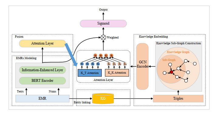
Diagnosis assistant is an effective way to reduce the workloads of professional doctors. The rich professional knowledge plays a crucial role in diagnosis. Therefore, it is important to introduce the relevant medical knowledge into diagnosis assistant. In this paper, diagnosis assistant is treated as a classification task, and a Graph-based Structural Knowledge-aware Network (GSKN) model is proposed to fuse Electronic Medical Records (EMRs) and medical knowledge graph. Considering that different information in EMRs affects the diagnosis results differently, the information in EMRs is categorized into general information, key information and numerical information, and is introduced to GSKN by adding an enhancement layer to the Bidirectional Encoder Representation from Transformers (BERT) model. The entities in EMRs are recognized, and Graph Convolutional Neural Networks (GCN) is employed to learn deep-level graph structure information and dynamic representation of these entities in the subgraphs. An interactive attention mechanism is utilized to fuse the enhanced textual representation and the deep representation of these subgraphs. Experimental results on Chinese Obstetric Electronic Medical Records (COEMRs) and open dataset C-EMRs demonstrate the effectiveness of our model.
Citation: Kunli Zhang, Bin Hu, Feijie Zhou, Yu Song, Xu Zhao, Xiyang Huang. Graph-based structural knowledge-aware network for diagnosis assistant[J]. Mathematical Biosciences and Engineering, 2022, 19(10): 10533-10549. doi: 10.3934/mbe.2022492
Diagnosis assistant is an effective way to reduce the workloads of professional doctors. The rich professional knowledge plays a crucial role in diagnosis. Therefore, it is important to introduce the relevant medical knowledge into diagnosis assistant. In this paper, diagnosis assistant is treated as a classification task, and a Graph-based Structural Knowledge-aware Network (GSKN) model is proposed to fuse Electronic Medical Records (EMRs) and medical knowledge graph. Considering that different information in EMRs affects the diagnosis results differently, the information in EMRs is categorized into general information, key information and numerical information, and is introduced to GSKN by adding an enhancement layer to the Bidirectional Encoder Representation from Transformers (BERT) model. The entities in EMRs are recognized, and Graph Convolutional Neural Networks (GCN) is employed to learn deep-level graph structure information and dynamic representation of these entities in the subgraphs. An interactive attention mechanism is utilized to fuse the enhanced textual representation and the deep representation of these subgraphs. Experimental results on Chinese Obstetric Electronic Medical Records (COEMRs) and open dataset C-EMRs demonstrate the effectiveness of our model.

| [1] | National Health and Family Planning Commission of the P. R. C., Guiding opinions of the General Office of the State Council on promoting the construction and development of medical consortium, Bulletin of The State Council of the People's Republic of China, 2017. |
| [2] | China's Ministry of Health, Basic specification of electronic medical records (trial), Chin. Med. Rec., 11 (2010), 64–65. |
| [3] |
R. S. Ledley, L. B. Lusted, Reasoning foundations of medical diagnosis: Symbolic logic, probability, and value theory aid our understanding of how physicians reason, Science, 130 (1959), 9–21. https://doi.org/10.1126/science.130.3366.9 doi: 10.1126/science.130.3366.9

|
| [4] |
E. H. Shortliffe, S. G. Axline, B. G. Buchanan, T. C. Merigan, S. N. Cohen, An artificial intelligence program to advise physicians regarding antimicrobial therapy, Comput. Biomed. Res., 6 (1973), 544–560. https://doi.org/10.1016/0010-4809(73)90029-3 doi: 10.1016/0010-4809(73)90029-3
|
| [5] | S. Mekruksavanich, Medical expert system based ontology for diabetes disease diagnosis, in 2016 7th IEEE International Conference on Software Engineering and Service Science (ICSESS), (2016), 383–389. https://doi.org/10.1109/ICSESS.2016.7883091 |
| [6] | K. Baati, T. M. Hamdani, A. M. Alimi, Diagnosis of lymphatic diseases using a naïve bayes style possibilistic classifier, in 2013 IEEE International Conference on Systems, Man, and Cybernetics, (2013), 4539–4542. https://doi.org/10.1109/SMC.2013.772 |
| [7] |
D. Çalişir, E. Dogantekin, A new intelligent hepatitis diagnosis system: PCA-LSSVM, Expert Syst. Appl., 38 (2011), 10705–10708. https://doi.org/10.1016/j.eswa.2011.01.014 doi: 10.1016/j.eswa.2011.01.014
|
| [8] |
A. F. Otoom, E. E. Abdallah, Y. Kilani, A. Kefaye, M. Ashour, Effective diagnosis and monitoring of heart disease, Int. J. Software Eng. Appl., 9 (2015), 143–156. https://doi.org/10.14257/ijseia.2015.9.1.12 doi: 10.14257/ijseia.2015.9.1.12
|
| [9] |
C. W. Liang, H. C. Yang, M. M. Islam, P. A. A. Nguyen, Y. T. Feng, Z. Y. Hou, et al., Predicting Hepatocellular Carcinoma with minimal features from electronic health records: Development of a deep learning model, JMIR Cancer, 7 (2021), e19812. https://doi.org/10.2196/19812 doi: 10.2196/19812
|
| [10] |
K. Kim, H. Yang, J. Yi, H. E. Son, J. Y. Ryu, Y. C. Kim, et al., Real-time clinical decision support based on recurrent neural networks for in-hospital acute kidney injury: External validation and model interpretation, J. Med. Int. Res., 23 (2021), e24120. https://doi.org/10.2196/24120 doi: 10.2196/24120
|
| [11] |
Y. Du, H. Wang, W. Cui, H. Zhu, Y. Guo, F. A. Dharejo, et al., Foodborne disease risk prediction using multigraph structural long short-term memory networks: Algorithm design and validation study, JMIR Med. Inf., 9 (2021), e29433. https://doi.org/10.2196/29433 doi: 10.2196/29433
|
| [12] | A. Sedik, M. Hammad, A. El-Samie, E. Fathi, B. B. Gupta, A. El-Latif, et al., Efficient deep learning approach for augmented detection of Coronavirus disease, Neural Comput. Appl., (2021), 1–18. https://doi.org/10.1007/s00521-020-05410-8. |
| [13] | K. Zhang, X. Zhao, L. Zhuang, Q. Xie, H. Zan, Knowledge-enabled diagnosis assistant based on obstetric EMRs and knowledge graph, in China National Conference on Chinese Computational Linguistics, Springer, 23 (2020), 444–457. https://doi.org/10.1007/978-3-030-63031-7_32 |
| [14] | J. Devlin, M. W. Chang, K. Lee, K. Toutanova, BERT: Pretraining of deep bidirectional transformers for language understanding, preprint, arXiv: 1810.04805. |
| [15] | A. Bordes, N. Usunier, A. Garcia-Duran, J. Weston, O. Yakhnenko, Translating embeddings for modeling multi-relational data, in Advances in Neural Information Processing Systems, 26 (2013), 1–9. https://dl.acm.org/doi/10.5555/2999792.2999923 |
| [16] | T. N. Kipf, M. Welling, Semi-supervised classification with graph convolutional networks, preprint, arXiv: 1609.02907. |
| [17] | A. Vaswani, N. Shazeer, N. Parmar, J. Uszkoreit, L. Jones, A. N. Gomez, et al., Attention is all you need, in Advances in Neural Information Processing Systems, 30 (2017), 1–11. https://dl.acm.org/doi/10.5555/3295222.3295349 |
| [18] | C. Qu, L. Yang, M. Qiu, W. B. Croft, Y. Zhang, M. Iyyer, BERT with history answer embedding for conversational question answering, in Proceedings of the 42nd International ACM SIGIR Conference on Research and Development in Information Retrieval, (2019), 1133–1136. https://doi.org/10.1145/3331184.3331341 |
| [19] |
Z. Yang, Y. Huang, Y. Jiang, Y. Sun, Y. J. Zhang, P. Luo, Clinical assistant diagnosis for electronic medical record based on convolutional neural network, Sci. Rep., 8 (2018), 1–9. https://doi.org/10.1038/s41598-018-24389-w doi: 10.1038/s41598-018-24389-w
|
| [20] | Y. Chen, Convolutional neural network for sentence classification, preprint, arXiv: 1408.5882. |
| [21] | S. Lai, L. Xu, K. Liu, J. Zhao, Recurrent convolutional neural networks for text classification, in Twenty-ninth AAAI Conference on Artificial Intelligence, (2015), 2267–2273. https://dl.acm.org/doi/abs/10.5555/2886521.2886636 |
| [22] | P. Zhou, W. Shi, J. Tian, Z. Qi, B. Li, H. Hao, et al., Attention-based bidirectional long short-term memory networks for relation classification, in Proceedings of the 54th Annual Meeting of the Association for Computational Linguistics, 2 (2016), 207–212. https://doi.org/10.18653/v1/P16-2034 |
| [23] | K. Zhang, C. Hu, Y. Song, H. Zan, Y. Zhao, W. Chu, Construction of Chinese obstetrics knowledge graph based on the multiple sources data, in Workshop on Chinese Lexical Semantics, (2022), 399–410. https://doi.org/10.1007/978-3-031-06547-7_31 |
| [24] | O. Byambasuren, Y. Yang, Z. Sui, D. Dai, B. Chang, S. Li, et al., Preliminary study on the construction of Chinese medical knowledge graph, J. Chin. Inf. Process, 10 (2019), 1–9. |
| [25] | H. Zan, Y. Han, Y. Fan, C. Niu, K. Zhang, Z. Sui, Construction and analysis of symptom knowledge base in Chinese, J. Chin. Inf. Process, 34 (2020), 30–37. |


Figures(7) / Tables(4)

Kunli Zhang, Bin Hu, Feijie Zhou, Yu Song, Xu Zhao, Xiyang Huang. Graph-based structural knowledge-aware network for diagnosis assistant[J]. Mathematical Biosciences and Engineering, 2022, 19(10): 10533-10549. doi: 10.3934/mbe.2022492


 DownLoad: