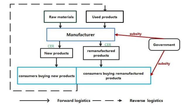
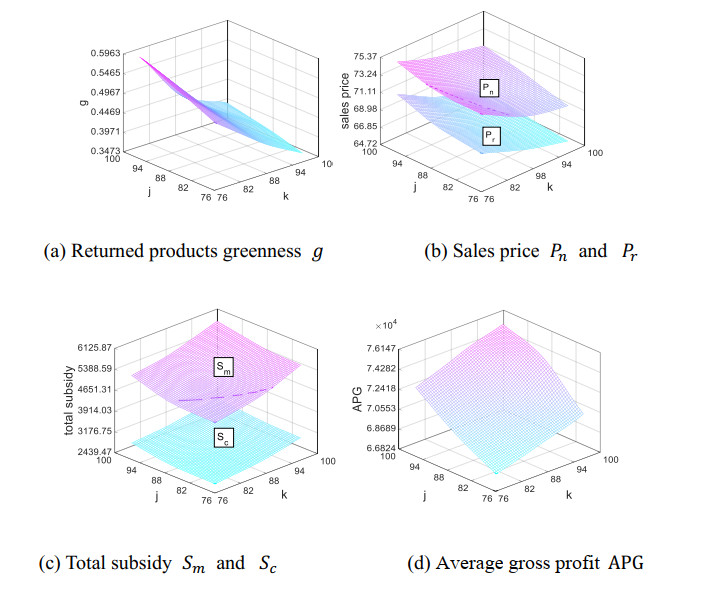
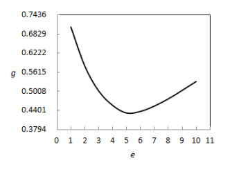
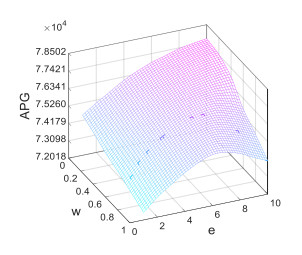
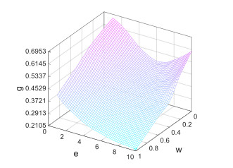
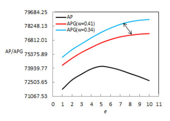
Under the uncertain market demand and quality level, a total profit model of green closed-loop supply chain system (GCL-SCS) considering corporate environmental responsibility (CER) and government differential weight subsidy (GDWS) is constructed. Based on incentive-compatibility theory, the optimal subsidy allocation policy and green investment level were explored. Fuzzy chance-constrained programming (FCCP) is used to clarify the uncertainty factors of this model; while genetic algorithm (GA) and CPLEX are used to find and compare a calculating example's approximate optimal solution about this model. The main calculating results indicate that: (1) Enterprises can make optimal recycling, production and sales strategies according to different potential demand; (2) Without government subsidy, enterprises' higher green investment level will reduce their average gross profit, increase the quality level of recycled products and decrease the recycling rate, hence reduce their environmental protection willingness; (3) Based on incentive-compatibility theory, when government subsidy weight is set as 0.34~0.41 for consumers, enterprises' higher green investment level will enhance their average gross profit, reduce the quality level of recycled products and increase the recycling rate, which will improve their environmental protection willingness; (4) Under uncertain environment, the combination of reasonable government subsidy policy and enterprises green investment can make up for the defect of enterprises green investment alone, maximize utilities of government and enterprises, and optimize the green closed loop supply chain.
Citation: Jianquan Guo, Guanlan Wang, Mitsuo Gen. Green closed-loop supply chain optimization strategy considering CER and incentive-compatibility theory under uncertainty[J]. Mathematical Biosciences and Engineering, 2022, 19(9): 9520-9549. doi: 10.3934/mbe.2022443
Under the uncertain market demand and quality level, a total profit model of green closed-loop supply chain system (GCL-SCS) considering corporate environmental responsibility (CER) and government differential weight subsidy (GDWS) is constructed. Based on incentive-compatibility theory, the optimal subsidy allocation policy and green investment level were explored. Fuzzy chance-constrained programming (FCCP) is used to clarify the uncertainty factors of this model; while genetic algorithm (GA) and CPLEX are used to find and compare a calculating example's approximate optimal solution about this model. The main calculating results indicate that: (1) Enterprises can make optimal recycling, production and sales strategies according to different potential demand; (2) Without government subsidy, enterprises' higher green investment level will reduce their average gross profit, increase the quality level of recycled products and decrease the recycling rate, hence reduce their environmental protection willingness; (3) Based on incentive-compatibility theory, when government subsidy weight is set as 0.34~0.41 for consumers, enterprises' higher green investment level will enhance their average gross profit, reduce the quality level of recycled products and increase the recycling rate, which will improve their environmental protection willingness; (4) Under uncertain environment, the combination of reasonable government subsidy policy and enterprises green investment can make up for the defect of enterprises green investment alone, maximize utilities of government and enterprises, and optimize the green closed loop supply chain.

| [1] |
M. S. Atabaki, M. Mohammadi, B. Naderi, New robust optimization models for closed-loop supply chain of durable products: Towards a circular economy, Comput. Ind. Eng., 146 (2020), 106520. https://doi.org/10.1016/j.cie.2020.106520 doi: 10.1016/j.cie.2020.106520

|
| [2] |
B. Khorshidvand, H. Soleimaniab, S. Sibdaric, M. M. S. Esfahanid, A hybrid modeling approach for green and sustainable closed-loop supply chain considering price, advertisement and uncertain demands, Comput. Ind. Eng., 157 (2021), 107326. https://doi.org/10.1016/j.cie.2021.107326 doi: 10.1016/j.cie.2021.107326
|
| [3] |
H. Liao, L. Li, Environmental sustainability EOQ model for closed-loop supply chain under market uncertainty: A case study of printer remanufacturing, Comput. Ind. Eng., 149 (2020), 106779. https://doi.org/10.1016/j.cie.2020.106525 doi: 10.1016/j.cie.2020.106525
|
| [4] |
R. Dominguez, B. Ponte, S. Cannella, J. M. Framinan, On the dynamics of closed-loop supply chains with capacity constraints, Comput. Ind. Eng., 128 (2019), 91-103. https://doi.org/10.1016/j.cie.2018.12.003 doi: 10.1016/j.cie.2018.12.003
|
| [5] |
H. Peng, N. Shen, H. Liao, H. Xue, Q. Wang, Uncertainty factors, methods, and solutions of closed-loop supply chain — A review for current situation and future prospects, J. Clean Prod., 254 (2020), 120032. https://doi.org/10.1016/j.jclepro.2020.120032 doi: 10.1016/j.jclepro.2020.120032
|
| [6] |
B. Zhu, B. Wen, S. Ji, R. Qiu, Coordinating a dual-channel supply chain with conditional value-at-risk under uncertainties of yield and demand, Comput. Ind. Eng., 139 (2020), 106181. https://doi.org/10.1016/j.cie.2019.106181 doi: 10.1016/j.cie.2019.106181
|
| [7] |
I. I. Almaraj, T. B. Trafalis, An integrated multi-echelon robust closed- loop supply chain under imperfect quality production, Int. J. Prod. Econ., 218 (2019), 212-227. https://doi.org/10.1016/j.ijpe.2019.04.035 doi: 10.1016/j.ijpe.2019.04.035
|
| [8] |
L. Wang, Q. Song, Pricing policies for dual-channel supply chain with green investment and sales effort under uncertain demand, Math Comput. Simul., 171 (2020), 79-93. https://doi.org/10.1016/j.matcom.2019.08.010 doi: 10.1016/j.matcom.2019.08.010
|
| [9] |
C. Li, L. Feng, S. Luo, Strategic introduction of an online recycling channel in the reverse supply chain with a random demand, J. Clean Prod., 236 (2019), 117683. https://doi.org/10.1016/j.jclepro.2019.117683 doi: 10.1016/j.jclepro.2019.117683
|
| [10] |
Y. Dai, L. Dou, H. Song, H. Y. Li, Two-way information sharing of uncertain demand forecasts in a dual-channel supply chain, Comput. Ind. Eng., 169 (2022), 108162. https://doi.org/10.1016/j.cie.2022.108162 doi: 10.1016/j.cie.2022.108162
|
| [11] |
X. Y. Zhu, Y. ZH. Cao, J. W. Wu, H. Liu, X. Q. Bei, Optimum operational schedule and accounts receivable financing in a production supply chain considering hierarchical industrial status and uncertain yield, Euro. J. Oper. Res., 302 (2022), 1142-1154. https://doi.org/10.1016/j.ejor.2022.02.008 doi: 10.1016/j.ejor.2022.02.008
|
| [12] |
L. J. Zeballos, M. I. Gomes, A. P. Barbosa-Povoa, A. Q. Novaisa, Addressing the uncertain quality and quantity of returns in closed-loop supply chains, Comput. Chem. Eng., 47 (2012), 237-247. https://doi.org/10.1016/j.compchemeng.2012.06.034 doi: 10.1016/j.compchemeng.2012.06.034
|
| [13] | M. Jeihoonian, M. K. Zanjani, M. Gendreaub, Closed-loop supply chain network design under uncertain quality status: Case of durable products, Int. J. Prod. Econ., 183 (2017), Part B, 470-486. https://doi.org/10.1016/j.ijpe.2016.07.023 |
| [14] |
J. Heydari, M. Ghasemi, A revenue sharing contract for reverse supply chain coordination under stochastic quality of returned products and uncertain remanufacturing capacity, J. Clean Prod., 197 (2018), 607-615. https://doi.org/10.1016/j.jclepro.2018.06.206 doi: 10.1016/j.jclepro.2018.06.206
|
| [15] |
A. Aminipour, Z. Bahroun, M. Hariga, Cyclic manufacturing and remanufacturing in a closed-loop supply chain, Sustain Prod. Consump., 25 (2021), 43-59. https://doi.org/10.1016/j.spc.2020.08.002 doi: 10.1016/j.spc.2020.08.002
|
| [16] |
Z. Ghelichi, M. Saidi-Mehrabad, M. S. Pishvaee, A stochastic programming approach toward optimal design and planning of an integrated green biodiesel supply chain network under uncertainty: A case study, Energy, 156 (2018), 661-687. https://doi.org/10.1016/j.energy.2018.05.103 doi: 10.1016/j.energy.2018.05.103
|
| [17] |
M. Farrokh, A. Azar, G. Jandaghi, E. Ahmadi, A novel robust fuzzy stochastic programming for closed loop supply chain network design under hybrid uncertainty, Fuzzy Set. Syst., 341 (2018), 69-91. https://doi.org/10.1016/j.fss.2017.03.019 doi: 10.1016/j.fss.2017.03.019
|
| [18] |
S. Ahmadi, S. H. Amin, An integrated chance-constrained stochastic model for a mobile phone closed-loop supply chain network with supplier selection, J. Clean Prod., 226 (2019), 988-1003. https://doi.org/10.1016/j.jclepro.2019.04.132 doi: 10.1016/j.jclepro.2019.04.132
|
| [19] |
M. Josefa, P. David, P. Raul, The effectiveness of a fuzzy mathematical programming approach for supply chain production planning with fuzzy demand, Int. J. Prod. Econ., 128 (2010), 136-143. https://doi.org/10.1016/j.ijpe.2010.06.007 doi: 10.1016/j.ijpe.2010.06.007
|
| [20] |
C. Lima, S. Relvas, A. Barbosa-Póvoab, Designing and planning the downstream oil supply chain under uncertainty using a fuzzy programming approach, Comput. Chem. Eng., 151 (2021), 107373. https://doi.org/10.1016/j.compchemeng.2021.107373 doi: 10.1016/j.compchemeng.2021.107373
|
| [21] |
F. Ziya-Gorabi, A. Ghodratnama, R. Tavakkoli-Moghaddam, M. S. Asadi-Lari, A new fuzzy tri-objective model for a home health care problem with green ambulance routing and congestion under uncertainty, Expert Syst. Appl., 201 (2022), 117093. https://doi.org/10.1016/j.eswa.2022.117093 doi: 10.1016/j.eswa.2022.117093
|
| [22] |
J. Ghahremani-Nahr, R. Kian, E. Sabetd, A robust fuzzy mathematical programming model for the closed-loop supply chain network design and a whale optimization solution algorithm, Expert Syst. Appl., 116 (2019), 454-471. https://doi.org/10.1016/j.eswa.2018.09.027 doi: 10.1016/j.eswa.2018.09.027
|
| [23] |
H. Jafar, R. Pooya, Integration of environmental and social responsibilities in managing supply chains: A mathematical modeling approach, Comput. Ind. Eng., 145 (2020), 106495. https://doi.org/10.1016/j.cie.2020.106495 doi: 10.1016/j.cie.2020.106495
|
| [24] |
J. Q. Guo, H. L. Yu, M. Gen, Research on green closed-loop supply chain with the consideration of double subsidy in e-commerce environment, Comput. Ind. Eng., 149 (2020), 106779. https://doi.org/10.1016/j.cie.2020.106779 doi: 10.1016/j.cie.2020.106779
|
| [25] |
J. Jian, B. Lia, N. Zhang, J. F. Su, Decision-making and coordination of green closed-loop supply chain with fairness concern, J. Clean Prod., 298 (2021), 126779. https://doi.org/10.1016/j.jclepro.2021.126779 doi: 10.1016/j.jclepro.2021.126779
|
| [26] |
Y. Liu, L. Ma, Y. k. Liu, A novel robust fuzzy mean-UPM model for green closed-loop supply chain network design under distribution ambiguity, Appl. Math. Model., 92 (2021), 99-135. https://doi.org/10.1016/j.apm.2020.10.042 doi: 10.1016/j.apm.2020.10.042
|
| [27] |
27. T. Asghari, A. A. Taleizadeh, F. Jolai, M. SadeghMoshtagh, Cooperative game for coordination of a green closed-loop supply chain, J. Clean Prod., 363 (2022), 132371. https://doi.org/10.1016/j.jclepro.2022.132371 doi: 10.1016/j.jclepro.2022.132371
|
| [28] |
J. Heydari, P. Rafiei, Integration of environmental and social responsibilities in managing supply chains: A mathematical modeling approach, Comput. Ind. Eng., 145 (2020), 106495. https://doi.org/10.1016/j.cie.2020.106495 doi: 10.1016/j.cie.2020.106495
|
| [29] |
Z. Feng, T. Xiao, D. J. Robb, Environmentally responsible closed-loop supply chain models with outsourcing and authorization options, J. Clean Prod., 278 (2021), 123791. https://doi.org/10.1016/j.jclepro.2020.123791 doi: 10.1016/j.jclepro.2020.123791
|
| [30] |
B. Marchi, S. Zanoni, L. E. Zavanella, M. Y. Jaber, Green supply chain with learning in production and environmental investments, IFAC-Papers OnLine, 51 (2018), 1738-1743. https://doi.org/10.1016/j.ifacol.2018.08.205 doi: 10.1016/j.ifacol.2018.08.205
|
| [31] |
Y. S. Huang, C. C. Fang, Y. A. Lin, Inventory management in supply chains with consideration of Logistics, green investment and different carbon emissions policies, Comput. Ind. Eng., 139 (2020), 106207. https://doi.org/10.1016/j.cie.2019.106207 doi: 10.1016/j.cie.2019.106207
|
| [32] |
Z. Hong, X. Guo, Green product supply chain contracts considering environmental responsibilities, Omega, 83 (2019), 155-166. https://doi.org/10.1016/j.omega.2018.02.010 doi: 10.1016/j.omega.2018.02.010
|
| [33] |
J. Cheng, B. Li, B. Gong, M. Cheng, L. Xu, The optimal power structure of environmental protection responsibilities transfer in remanufacturing supply chain, J. Clean Prod., 153 (2017), 558-569. https://doi.org/10.1016/j.jclepro.2016.02.097 doi: 10.1016/j.jclepro.2016.02.097
|
| [34] |
X. Y. Han, T. Y. Cao, Study on corporate environmental responsibility measurement method of energy consumption and pollution discharge and its application in industrial parks, J. Clean Prod., 326 (2022), 129359. https://doi.org/10.1016/j.jclepro.2021.129359 doi: 10.1016/j.jclepro.2021.129359
|
| [35] |
D. Y. Yang, D. P. Song, C. F. Li, Environmental responsibility decisions of a supply chain under different channel leaderships, Environ. Technol. Inno., 26 (2022), 102212. https://doi.org/10.1016/j.eti.2021.102212 doi: 10.1016/j.eti.2021.102212
|
| [36] |
W. Wu, Q. Zhang, Z. Liang, Environmentally responsible closed-loop supply chain models for joint environmental responsibility investment, recycling and pricing decisions, J. Clean Prod., 259 (2020), 120776. https://doi.org/10.1016/j.jclepro.2020.120776 doi: 10.1016/j.jclepro.2020.120776
|
| [37] |
R. Yang, W. S. Tang, J. X. Zhang, Government subsidies for green technology development under uncertainty, Euro J. Oper. Res., 286 (2020), 726-739. https://doi.org/10.1016/j.eti.2021.102212 doi: 10.1016/j.eti.2021.102212
|
| [38] | S. Zheng, L. H. Yu, The government's subsidy strategy of carbon-sink fishery based on evolutionary game, Energy, 254 (2022), Part B, 124282. https://doi.org/10.1016/j.energy.2022.124282 |
| [39] |
W. T. Chen, Z. H. Hu, Using evolutionary game theory to study governments and manufacturers' behavioral strategies under various carbon taxes and subsidies, J. Clean Prod., 201 (2018), 123-141. https://doi.org/10.1016/j.jclepro.2018.08.007 doi: 10.1016/j.jclepro.2018.08.007
|
| [40] | M. C. Cohen, R. Lobel, G. Perakis, The impact of demand uncertainty on consumer subsidies for green technology adoption, Manage. Sci., 62 (2016), 1235-1258. https://doi.org/http://hdl.handle.net/1721.1/111095 |
| [41] |
J. S. Bian, G. Q. Zhang, G. H. Zhou, Manufacturer vs. Consumer Subsidy with Green Technology Investment and Environmental Concern, Euro J. Oper. Res., 287 (2020), 832-843. https://doi.org/10.1016/j.ejor.2020.05.014 doi: 10.1016/j.ejor.2020.05.014
|
| [42] |
Y. W. Deng, N. Li, Zh. B. Jiang, X. Q. Xie, N. Kong, Optimal differential subsidy policy design for a workload-imbalanced outpatient care network, Omega, 99 (2021), 102194. https://doi.org/10.1016/j.omega.2020.102194 doi: 10.1016/j.omega.2020.102194
|
| [43] | W. Wang, S. J. Hao, W. He, M. AbdulkadirMohamed, Carbon emission reduction decisions in construction supply chain based on differential game with government subsidies, Build Environ., (2022), 109149. https://doi.org/10.1016/j.buildenv.2022.109149 |
| [44] |
S. Chen, J. F. Su, Y. B. Wu, F. L. Zhou, Optimal production and subsidy rate considering dynamic consumer green perception under different government subsidy orientations, Comput. Ind. Eng., 168 (2022), 108073. https://doi.org/10.1016/j.cie.2022.108073 doi: 10.1016/j.cie.2022.108073
|
| [45] |
A. Suliman, H. Otrok, R. Mizouni, A greedy-proof incentive-compatible mechanism for group recruitment in mobile crowd sensing, Future Gener. Comp. Syst., 101 (2019), 1158-1167. https://doi.org/10.1016/j.future.2019.07.060 doi: 10.1016/j.future.2019.07.060
|
| [46] |
I. E. Nielsen, S. Majumder, S. S. Sana, S. Saha, Comparative analysis of government incentives and game structures on single and two-period green supply chain, J. Clean Prod., 235 (2019), 1371-1398. https://doi.org/10.1016/j.jclepro.2019.06.168 doi: 10.1016/j.jclepro.2019.06.168
|
| [47] |
W. Wang, Y. Zhang, W. Zhang, Incentive mechanisms in a green supply chain under demand uncertainty, J. Clean Prod., 279 (2021), 123636. https://doi.org/10.1016/j.jclepro.2020.123636 doi: 10.1016/j.jclepro.2020.123636
|
| [48] |
Z. Qu, H. Raff, N. Schmitt, Incentives through inventory control in supply chains, Int. J. Ind. Org., 59 (2018), 486-513. https://doi.org/10.1016/j.ijindorg.2018.06.001 doi: 10.1016/j.ijindorg.2018.06.001
|
| [49] |
Z. Wang, Z. Wang, N. Tahir, Study of synergetic development in straw power supply chain: Straw price and government subsidy as incentive, Energy Policy, 146 (2020), 111788. https://doi.org/10.1016/j.enpol.2020.111788 doi: 10.1016/j.enpol.2020.111788
|
| [50] |
Y. H. Zhang, Y. Wang, The impact of government incentive on the two competing supply chains under the perspective of Corporation Social Responsibility: A case study of Photovoltaic industry, J. Clean Prod., 154 (2017), 102-113. https://doi.org/10.1016/j.jclepro.2017.03.127 doi: 10.1016/j.jclepro.2017.03.127
|
| [51] |
H. Y. Guo, N. C. Yannelis, Incentive compatibility under ambiguity, J. Econo. Theory., 73 (2022), 565-593. https://doi.org/10.1007/s00199-020-01304-x doi: 10.1007/s00199-020-01304-x
|
| [52] |
S. Barberà, D. Berga, B. Moreno, Restricted environments and incentive compatibility in interdependent values models, Game Econo. Behav., 131 (2022), 1-28. https://doi.org/10.1016/j.geb.2021.10.008 doi: 10.1016/j.geb.2021.10.008
|
| [53] |
Y. H. Feng, S. Deb, G. G. Wang, A. H. Alavi, Monarch butterfly optimization: A comprehensive review, Expert Syst. Appl., 168 (2021), 114418. https://doi.org/10.1016/j.eswa.2020.114418 doi: 10.1016/j.eswa.2020.114418
|
| [54] |
G. G. Wang, S. Deb, Z. H. Cui, Monarch butterfly optimization, Neural Comput. Appl., 31 (2019), 1995-2014. https://doi.org/10.1007/s00521-015-1923-y doi: 10.1007/s00521-015-1923-y
|
| [55] |
H. F. Rahman, M. N. Janardhanan, L. P. Chuen, S. G. Ponnambalam, Flowshop scheduling with sequence dependent setup times and batch delivery in supply chain, Comput. Ind. Eng., 158 (2021), 107378. https://doi.org/10.1016/j.cie.2021.107378 doi: 10.1016/j.cie.2021.107378
|
| [56] |
A. Chouar, S.Tetouani, A.Soulhi, J. Elalami, Performance improvement in physical internet supply chain network using hybrid framework, IFAC-Papers OnLine, 54 (2121), 593-598. https://doi.org/10.1016/j.ifacol.2021.10.514 doi: 10.1016/j.ifacol.2021.10.514
|
| [57] |
Y. T. Yang, H. L. Chen, A. A. Heidari, A. HGandom, Hunger games search: Visions, conception, implementation, deep analysis, perspectives, and towards performance shifts, Expert Syst. Appl., 177 (2021), 114864. https://doi.org/10.1016/j.eswa.2021.114864 doi: 10.1016/j.eswa.2021.114864
|
| [58] |
H. Nguyen, X. N. Bui, A novel hunger games search optimization-based artificial neural network for predicting ground vibration intensity induced by mine blasting, Nat. Resour. Res., 30 (2021), 3865-3880. https://doi.org/10.1007/s11053-021-09903-8 doi: 10.1007/s11053-021-09903-8
|
| [59] |
R. D. Ambrosio, S. D. Giovacchino, Nonlinear stability issues for stochastic Runge-Kutta methods, Sci. Num. Simul., 94 (2021), 105549. https://doi.org/10.1016/j.cnsns.2020.105549 doi: 10.1016/j.cnsns.2020.105549
|
| [60] |
B. B. Shi, HuaYe, L. Zheng, J. C. Lyu, C. Chen, A. A. Heidari, Z. Y. Hu, H. L. Chen, P. L. Wu, Evolutionary warning system for COVID-19 severity: Colony predation algorithm enhanced extreme learning machine, Comput. Biol. Med., 136 (2021), 104698. https://doi.org/10.1016/j.compbiomed.2021.104698 doi: 10.1016/j.compbiomed.2021.104698
|
| [61] |
A. S. Mashaleh, N. F. B. Ibrahim, M. A. Al-Betar, H. M. J. Mustafa, Q. M. Yaseenc, Detecting spam email with machine learning optimized with Harris Hawks optimizer (HHO) algorithm, Procedia Comput. Sci., 201 (2022), 659-664. https://doi.org/10.1016/j.procs.2022.03.087 doi: 10.1016/j.procs.2022.03.087
|
| [62] | M. Gen, R.W. Cheng, L. Lin, "Network Models and Optimization: Multiple Objective Genetic Algorithm Approach", 710pp, Springer, London, (2008). |
| [63] | X. X. Liu, J. Q. Guo, C. J. Liang, Joint Design model of multi-period reverse logistics network with the consideration of carbon emissions for e-commerce enterprises, Proceed. ICEBE2015, (2015), 428-433. https://doi.org/10.1109/ICEBE.2015.78 |
| [64] |
N. Sahebjamnia, A. M. Fathollahi-Fard, M. Hajiaghaei-Keshteli, Sustainable tire closed-loop supply chain network design: Hybrid meta-heuristic algorithms for large-scale networks, J. Clean Prod., 196 (2018), 273-296. https://doi.org/10.1016/j.jclepro.2018.05.245 doi: 10.1016/j.jclepro.2018.05.245
|
| [65] |
J. Y. Feng, B. Y. Yuan, X. Li, D. Tian, W. S. Mu, Evaluation on risks of sustainable supply chain based on optimized BP neural networks in fresh grape industry, Agriculture, 183 (2021), 105988. https://doi.org/10.1016/j.compag.2021.105988 doi: 10.1016/j.compag.2021.105988
|
| [66] |
S. X. Zhao, Y. C. Wang, Z. Y. Jiang, T. S. Hu, F. M. Chu, Research on emergency distribution optimization of mobile power for electric vehicle in photovoltaic-energy storage-charging supply chain under the energy blockchain, Energy Rep., 8 (2022), 6815-6825. https://doi.org/10.1016/j.egyr.2022.05.010 doi: 10.1016/j.egyr.2022.05.010
|
| [67] |
X. Y. Wang, J. Q. Guo, Optimal strategies of different quality level of returned Products for manufacturing/remanufacturing enterprises under carbon tax, Resour. Develop. mkt., 33 (2017), 59-63. https://doi.org/10.3969/j.issn.1005-8141.2017.01.011 doi: 10.3969/j.issn.1005-8141.2017.01.011
|
| [68] |
J. Q. Guo, L. He, M. Gen, Optimal strategies for the closed-loop supply chain with the consideration of supply disruption and subsidy policy, Comput. Ind. Eng., 128 (2019), 886-893. https://doi.org/10.1016/j.cie.2018.10.029 doi: 10.1016/j.cie.2018.10.029
|
| [69] |
N. Wan, D. Hong, The impacts of subsidy policies and transfer pricing policies on the closed-loop supply chain with dual collection channels, J. Clean Prod., 224 (2019), 881-891. https://doi.org/10.1016/j.jclepro.2019.03.274 doi: 10.1016/j.jclepro.2019.03.274
|
| [70] |
J. Q. Guo, Y. Gao, Optimal strategies for manufacturing/remanufacturing system with the consideration of recycled products, Comput. Ind. Eng., 89 (2015), 226-234. https://doi.org/10.1016/j.cie.2014.11.020 doi: 10.1016/j.cie.2014.11.020
|
| [71] |
Y. Yu, X. Han, G. Hu, Optimal production for manufacturers considering consumer environmental awareness and green subsidies, Int. J. Prod. Econ., 182 (2016), 397-408. https://doi.org/10.1016/j.cie.2022.108073 doi: 10.1016/j.cie.2022.108073
|
| [72] |
X. Gu, L. Zhou, H. Huang, X. Shi, Electric vehicle battery secondary use under government subsidy: A closed-loop supply chain perspective, Int. J. Prod. Econ., 234 (2021), 108035. https://doi.org/10.1016/j.ijpe.2021.108035 doi: 10.1016/j.ijpe.2021.108035
|
| [73] |
N. Wang, Y. Song, Q. He, T. Jia, Competitive dual-collecting regarding consumer behavior and coordination in closed-loop supply chain, Comput. Ind. Eng., 144 (2020), 106481. https://doi.org/10.1016/j.cie.2020.106481 doi: 10.1016/j.cie.2020.106481
|
| [74] |
S. M. Hosseini-Motlagh, M. Johari, S. Ebrahimi, P. Rogetzer, Competitive channels coordination in a closed-loop supply chain based on energy-saving effort and cost-tariff contract, Comput. Ind. Eng., 149 (2020), 106763. https://doi.org/10.1016/j.cie.2020.106763 doi: 10.1016/j.cie.2020.106763
|
| [75] |
J. Q. Guo, Y. D. Kao, H. Huang, A manufacturing/remanufacturing system with the consideration of required quality of end-of-used products, Indus. Eng. Mgt. Syst., 9 (2010), 204-214. https://doi.org/10.7232/iems.2010.9.3.204 doi: 10.7232/iems.2010.9.3.204
|
| [76] |
Y. Wu, R. Lu, J. Yang, R. Wang, H. Xu, C. Jiang, F. Xu, Government-led low carbon incentive model of the online shopping supply chain considering the O2O model, J. Clean Prod., 279 (2021), 123271. https://doi.org/10.1016/j.jclepro.2020.123271 doi: 10.1016/j.jclepro.2020.123271
|
| [77] |
X. Wan, X. Qie, Poverty alleviation ecosystem evolutionary game on smart supply chain platform under the government financial platform incentive mechanism, J. Comput. Appl. Math., 372 (2020), 112595. https://doi.org/10.1016/j.cam.2019.112595 doi: 10.1016/j.cam.2019.112595
|
| [78] |
J. Bian, G. Zhang, G. Zhou, Manufacturer vs. Consumer subsidy with green technology investment and environmental concern, Euro. J. Oper. Res., 287 (2020), 832-843. https://doi.org/10.1016/j.ejor.2020.05.014 doi: 10.1016/j.ejor.2020.05.014
|
| [79] |
W. Wu, Q. Zhang, Z. Liang, Environmentally responsible closed-loop supply chain models for joint environmental responsibility investment, recycling and pricing decisions, J. Clean Prod., 259 (2020), 120776. https://doi.org/10.1016/j.jclepro.2020.120776 doi: 10.1016/j.jclepro.2020.120776
|
| [80] |
S. Nayeri, M. M. Paydar, E. Asadi-Gangraj, S. Emami, Multi-objective fuzzy robust optimization approach to sustainable closed-loop supply chain network design, Comput. Ind. Eng., 148 (2020), 106716. https://doi.org/10.1016/j.cie.2020.106716 doi: 10.1016/j.cie.2020.106716
|
| [81] |
K. Bhattacharya, S. D. Kumar, A robust two layer green supply chain modelling under performance based fuzzy game theoretic approach, Comput. Ind. Eng., 152 (2021), 107005. https://doi.org/10.1016/j.cie.2020.107005 doi: 10.1016/j.cie.2020.107005
|
| [82] |
M. Yavari, S. Isvandi, Integrated decision making for parts ordering and scheduling of jobs on two-stage assembly problem in three level supply chain, J. Manuf. Syst., 46 (2018), 137-151. https://doi.org/10.1016/j.jmsy.2017.12.002 doi: 10.1016/j.jmsy.2017.12.002
|
| [83] |
J. Wu, Y. Ding, L. Shi, Mathematical modeling and heuristic approaches for a multi-stage car sequencing problem, Comput. Ind. Eng., 152 (2021), 107008. https://doi.org/10.1016/j.cie.2020.107008 doi: 10.1016/j.cie.2020.107008
|
| [84] |
M. Hamdi, M. Zaied, Resource allocation based on hybrid genetic algorithm and particle swarm optimization for D2D multicast communications, Appl. Soft Comput., 83 (2019), 105605. https://doi.org/10.1016/j.asoc.2019.105605 doi: 10.1016/j.asoc.2019.105605
|
| [85] |
A. Afzal, M., K. Ramis, Multi-objective optimization of thermal performance in battery system using genetic and particle swarm algorithm combined with fuzzy logics, J. Energy Stor., 32 (2020), 101815. https://doi.org/10.1016/j.est.2020.101815 doi: 10.1016/j.est.2020.101815
|
| [86] |
M. Gen, L. Lin, Y.S. Yun, H. Inoue, Recent advances in hybrid priority-based genetic algorithms for logistics and SCM network design, Comput. Ind. Eng., 115 (2018), 394-412. https://doi.org/10.1016/j.cie.2018.08.025 doi: 10.1016/j.cie.2018.08.025
|
| [87] |
G. Ahn, S. Hur, Efficient genetic algorithm for feature selection for early time series classification, Comput. Ind. Eng., 142 (2020), 106345. https://doi.org/10.1016/j.cie.2020.106345 doi: 10.1016/j.cie.2020.106345
|
| [88] |
A. Rostami, M. M. Paydar, E. Asadi-Gangraj, A hybrid genetic algorithm for integrating virtual cellular manufacturing with supply chain management considering new product development, Comput. Ind. Eng., 145 (2020), 106565. https://doi.org/10.1016/j.cie.2020.106565 doi: 10.1016/j.cie.2020.106565
|

Figures(9) / Tables(6)

Jianquan Guo, Guanlan Wang, Mitsuo Gen. Green closed-loop supply chain optimization strategy considering CER and incentive-compatibility theory under uncertainty[J]. Mathematical Biosciences and Engineering, 2022, 19(9): 9520-9549. doi: 10.3934/mbe.2022443


 DownLoad: