The adoption of Big Data Analysis (BDA) has become popular among firms since it creates evidence for decision-making by managers. However, the adoption of BDA continues to be poor among small and medium enterprises (SMEs). Therefore, this study adopted the Technology-Organization-Environment (TOE) framework to identify the drivers of readiness to adopt BDA among SMEs. Chi-square automatic interaction detection (CHAID), Bayesian network, neural network, and C5.0 algorithms of data mining were utilized to analyze data collected from 240 Vietnamese managers of SMEs. The evaluation model identified the C5.0 algorithm as the best model, with accurate results for the prediction of factors influencing the readiness to adopt BDA among SMEs. The findings revealed management support, data quality, firm size, data security and cost to be the fundamental factors influencing BDA adoption readiness. Moreover, the results identified the service sector as having a higher level of readiness toward the adoption of BDA compared to the manufacturing sector. The findings are imperative for the enhancement of the decision-making process and advancement of comprehension of the determinants of BDA adoption among SMEs by researchers, managers, providers and policymakers.
Citation: Nguyen Thi Giang, Shu-Yi Liaw. An application of data mining algorithms for predicting factors affecting Big Data Analysis adoption readiness in SMEs[J]. Mathematical Biosciences and Engineering, 2022, 19(8): 8621-8647. doi: 10.3934/mbe.2022400
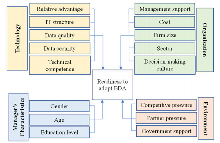
The adoption of Big Data Analysis (BDA) has become popular among firms since it creates evidence for decision-making by managers. However, the adoption of BDA continues to be poor among small and medium enterprises (SMEs). Therefore, this study adopted the Technology-Organization-Environment (TOE) framework to identify the drivers of readiness to adopt BDA among SMEs. Chi-square automatic interaction detection (CHAID), Bayesian network, neural network, and C5.0 algorithms of data mining were utilized to analyze data collected from 240 Vietnamese managers of SMEs. The evaluation model identified the C5.0 algorithm as the best model, with accurate results for the prediction of factors influencing the readiness to adopt BDA among SMEs. The findings revealed management support, data quality, firm size, data security and cost to be the fundamental factors influencing BDA adoption readiness. Moreover, the results identified the service sector as having a higher level of readiness toward the adoption of BDA compared to the manufacturing sector. The findings are imperative for the enhancement of the decision-making process and advancement of comprehension of the determinants of BDA adoption among SMEs by researchers, managers, providers and policymakers.

| [1] |
I. Yaqoob, I. A. T. Hashem, A. Gani, S. Mokhtar, E. Ahmed, N. B. Anuar, et al., Big data: from beginning to future, Int. J. Inf. Manage., 36 (2016), 1231-1247. https://doi.org/10.1016/j.ijinfomgt.2016.07.009 doi: 10.1016/j.ijinfomgt.2016.07.009

|
| [2] |
S. S. Alrumiah, M. Hadwan, Implementing big data analytics in e-commerce: Vendor and customer view, IEEE Access, 9 (2021), 37281-37286. https://doi.org/10.1109/ACCESS.2021.3063615 doi: 10.1109/ACCESS.2021.3063615
|
| [3] |
T. M. Le, S. Y. Liaw, Effects of pros and cons of applying big data analytics to consumers' responses in an e-commerce context, Sustainability, 9 (2017), 1-19. https://doi.org/10.3390/su9050798 doi: 10.3390/su9050798
|
| [4] |
M. Janssen, H. van der Voort, A. Wahyudi, Factors influencing big data decision-making quality, J. Bus. Res., 70 (2017), 338-345. https://doi.org/10.1016/j.jbusres.2016.08.007 doi: 10.1016/j.jbusres.2016.08.007
|
| [5] |
G. Wang, A. Gunasekaran, E. W. T. Ngai, T. Papadopoulos, Big data analytics in logistics and supply chain management: Certain investigations for research and applications, Int. J. Prod. Econ., 176 (2016), 98-110. https://doi.org/10.1016/j.ijpe.2016.03.014 doi: 10.1016/j.ijpe.2016.03.014
|
| [6] |
S. Tiwari, H. M. Wee, Y. Daryanto, Big data analytics in supply chain management between 2010 and 2016: Insights to industries, Comput. Ind. Eng., 115 (2018), 319-330. https://doi.org/10.1016/j.cie.2017.11.017 doi: 10.1016/j.cie.2017.11.017
|
| [7] |
S. Akter, S. F. Wamba, A. Gunasekaran, R. Dubey, S. J. Childe, How to improve firm performance using big data analytics capability and business strategy alignment?, Int. J. Prod. Econ., 182 (2016), 113-131. https://doi.org/10.1016/j.ijpe.2016.08.018 doi: 10.1016/j.ijpe.2016.08.018
|
| [8] |
P. Mikalef, M. Boura, G. Lekakos, J. Krogstie, Big data analytics and firm performance: Findings from a mixed-method approach, J. Bus. Res., 98 (2019), 261-276. https://doi.org/10.1016/j.jbusres.2019.01.044 doi: 10.1016/j.jbusres.2019.01.044
|
| [9] |
P. Maroufkhani, M. L. Tseng, M. Iranmanesh, W. K. W. Ismail, H. Khalid, Big data analytics adoption: Determinants and performances among small to medium-sized enterprises, Int. J. Inf. Manage., 54 (2020), 1-15. https://doi.org/10.1016/j.ijinfomgt.2020.102190 doi: 10.1016/j.ijinfomgt.2020.102190
|
| [10] |
Z. Xu, G. L. Frankwick, E. Ramirez, Effects of big data analytics and traditional marketing analytics on new product success: A knowledge fusion perspective, J. Bus. Res., 69 (2016), 1562-1566. https://doi.org/10.1016/j.jbusres.2015.10.017 doi: 10.1016/j.jbusres.2015.10.017
|
| [11] |
S. Mandal, An examination of the importance of big data analytics in supply chain agility development, Manag. Res. Rev., 41 (2018), 1201-1219. https://doi.org/10.1108/MRR-11-2017-0400 doi: 10.1108/MRR-11-2017-0400
|
| [12] |
L. Wang, M. Yang, Z. H. Pathan, S. Salam, K. Shahzad, J. Zeng, Analysis of influencing ffactors of Big Data Adoption in Chinese enterprises using DANP technique, Sustainability, 10 (2018), 1-16. https://doi.org/10.3390/su10113956 doi: 10.3390/su10113956
|
| [13] | B. Marr, Big Data in Practice: How 45 Successful Companies Used Big Data Analytics to Deliver Extraordinary Results, Wiley, 2016. https://doi.org/10.1002/9781119278825 |
| [14] |
A. Alharthi, V. Krotov, M. Bowman, Addressing barriers to big data, Bus. Horiz., 60 (2017), 285-292. https://doi.org/10.1016/j.bushor.2017.01.002 doi: 10.1016/j.bushor.2017.01.002
|
| [15] |
P. Tabesh, E. Mousavidin, S. Hasani, Implementing big data strategies: A managerial perspective, Bus. Horiz., 62 (2019), 347-358. https://doi.org/10.1016/j.bushor.2019.02.001 doi: 10.1016/j.bushor.2019.02.001
|
| [16] |
S. Venkatraman, R. Venkatraman, Big data security challenges and strategies, AIMS Math., 4 (2019), 860-879. https://doi.org/10.3934/math.2019.3.860 doi: 10.3934/math.2019.3.860
|
| [17] |
S. Coleman, R. Göb, G. Manco, A. Pievatolo, X. Tort-Martorell, M. S. Reis, How can SMEs benefit from big data? Challenges and a path forward, Qual. Reliab. Eng. Int., 32 (2016), 2151-2164. https://doi.org/10.1002/qre.2008 doi: 10.1002/qre.2008
|
| [18] |
C. O'Connor, S. Kelly, Facilitating knowledge management through filtered big data: SME competitiveness in an agri-food sector, J. Knowl. Manag., 21 (2017), 156-179. https://doi.org/10.1108/JKM-08-2016-0357 doi: 10.1108/JKM-08-2016-0357
|
| [19] |
P. Del Vecchio, A. Di Minin, A. M. Petruzzelli, U. Panniello, S. Pirri, Big data for open innovation in SMEs and large corporations: Trends, opportunities, and challenges, Creat. Innov. Manag., 27 (2018), 6-22. https://doi.org/10.1111/caim.12224 doi: 10.1111/caim.12224
|
| [20] | W. Noonpakdee, A. Phothichai, T. Khunkornsiri, Big data implementation for small and medium enterprises, in 2018 27th Wireless and Optical Communication Conference (WOCC), Hualien, Taiwan, (2018), 1-5. https://doi.org/10.1109/WOCC.2018.8372725 |
| [21] |
M. H. Chuah, R. Thurusamry, Challenges of big data adoption in Malaysia SMEs based on Lessig's modalities: A systematic review, Cogent. Bus. Manage., 8 (2021), 81-91. https://doi.org/10.1080/23311975.2021.1968191 doi: 10.1080/23311975.2021.1968191
|
| [22] |
S. K. Mangla, R. Raut, V. S. Narwane, Z. Zhang, P. Priyadarshinee, Mediating effect of big data analytics on project performance of small and medium enterprises, J. Enterp. Inf. Manag., 34 (2020), 168-198. https://doi.org/10.1108/JEIM-12-2019-0394 doi: 10.1108/JEIM-12-2019-0394
|
| [23] |
J. H. Park, Y. B. Kim, Factors activating big data adoption by Korean firms, J. Comput. Inf. Syst., 61 (2021), 285-293. https://doi.org/10.1080/08874417.2019.1631133 doi: 10.1080/08874417.2019.1631133
|
| [24] | L. G. Tornatzky, M. Fleischer, The Processes of Technological Innovation, Lexington Books, Massachusetts, 1990. |
| [25] |
D. Grant, B. Yeo, A global perspective on tech investment, financing, and ICT on manufacturing and service industry performance, Int. J. Inf. Manag., 43 (2018), 130-145. https://doi.org/10.1016/j.ijinfomgt.2018.06.007 doi: 10.1016/j.ijinfomgt.2018.06.007
|
| [26] |
R. Y. Zhong, S. T. Newman, G. Q. Huang, S. Lan, Big Data for supply chain management in the service and manufacturing sectors: Challenges, opportunities, and future perspectives, Comput. Ind. Eng., 101 (2016), 572-591. https://doi.org/10.1016/j.cie.2016.07.013 doi: 10.1016/j.cie.2016.07.013
|
| [27] |
M. K. Saggi, S. Jain, A survey towards an integration of big data analytics to big insights for value-creation, Inf. Proc. Manag., 54 (2018), 758-790. https://doi.org/10.1016/j.ipm.2018.01.010 doi: 10.1016/j.ipm.2018.01.010
|
| [28] |
S. F. Wamba, A. Gunasekaran, S. Akter, S. J. f. Ren, R. Dubey, S. J. Childe, Big data analytics and firm performance: Effects of dynamic capabilities, J. Bus. Res., 70 (2017), 356-365. https://doi.org/10.1016/j.jbusres.2016.08.009 doi: 10.1016/j.jbusres.2016.08.009
|
| [29] |
S. Dash, S. K. Shakyawar, M. Sharma, S. Kaushik, Big data in healthcare: management, analysis and future prospects, J. Big Data, 6 (2019), 1-25. https://doi.org/10.1186/s40537-019-0217-0 doi: 10.1186/s40537-019-0217-0
|
| [30] |
E. Yadegaridehkordi, M. Nilashi, L. Shuib, M. Hairul Nizam Bin Md Nasir, S. Asadi, S. Samad, et al., The impact of big data on firm performance in hotel industry, Electron. Commer. Res. Appl., 40 (2020), 1-32. https://doi.org/10.1016/j.elerap.2019.100921 doi: 10.1016/j.elerap.2019.100921
|
| [31] |
R. Dubey, A. Gunasekaran, S. J. Childe, Big data analytics capability in supply chain agility: The moderating effect of organizational flexibility, Manag. Decis., 57 (2019), 2092-2112. https://doi.org/10.1108/MD-01-2018-0119 doi: 10.1108/MD-01-2018-0119
|
| [32] |
S. Wang, H. Wang, Big data for small and medium-sized enterprises (SME): a knowledge management model, J. Knowl. Manag., 24 (2020), 881-897. https://doi.org/10.1108/JKM-02-2020-0081 doi: 10.1108/JKM-02-2020-0081
|
| [33] |
N. Mahdi, R. Javaneh, S. Mahmoud, The impact of big data adoption on SMEs performance, Res. Sq., 9 (2020), 1-12. https://doi.org/10.21203/rs.3.rs-66047/v1 doi: 10.21203/rs.3.rs-66047/v1
|
| [34] |
A. Lutfi, A. Alsyouf, M. A. Almaiah, M. Alrawad, A. A. K. Abdo, A. L. Al-Khasawneh, et al., Factors influencing the adoption of big data analytics in the digital transformation era: Case study of Jordanian SMEs, Sustainability, 14 (2022), 1-17. https://doi.org/10.3390/su14031802 doi: 10.3390/su14031802
|
| [35] |
S. Sun, C. G. Cegielski, L. Jia, D. J. Hall, Understanding the factors affecting the organizational adoption of big data, J. Comput. Inf. Syst., 58 (2016), 193-203. https://doi.org/10.1080/08874417.2016.1222891 doi: 10.1080/08874417.2016.1222891
|
| [36] |
P. Maroufkhani, R. Wagner, W. K. Wan Ismail, M. B. Baroto, M. Nourani, Big data analytics and firm performance: A systematic review, Information, 10 (2019), 1-21. https://doi.org/10.3390/info10070226 doi: 10.3390/info10070226
|
| [37] |
M. I. Baig, L. Shuib, E. Yadegaridehkordi, Big data adoption: State of the art and research challenges, Inf. Process. Manag., 56 (2019), 1-18. https://doi.org/10.1016/j.ipm.2019.102095 doi: 10.1016/j.ipm.2019.102095
|
| [38] |
S. Gupta, H. W. Kim, Linking structural equation modeling to Bayesian networks: Decision support for customer retention in virtual communities, Eur. J. Oper. Res., 190 (2008), 818-833. https://doi.org/10.1016/j.ejor.2007.05.054 doi: 10.1016/j.ejor.2007.05.054
|
| [39] |
P. F. Hsu, S. Ray, Y. Y. Li-Hsieh, Examining cloud computing adoption intention, pricing mechanism, and deployment model, Int. J. Inf. Manage., 34 (2014), 474-488. https://doi.org/10.1016/j.ijinfomgt.2014.04.006 doi: 10.1016/j.ijinfomgt.2014.04.006
|
| [40] | J. H. Park, M. K. Kim, J. H. Paik, The factors of technology, organization and environment influencing the adoption and usage of big data in korean firms, in 26th European Regional Conference of the Interational Telecommunications Society, Madrid, Spain, 24-27 June, 3 (2015), 121-129. |
| [41] |
Y. Lai, H. Sun, J. Ren, Understanding the determinants of big data analytics (BDA) adoption in logistics and supply chain management, Int. J. Logis. Manag., 29 (2018), 676-703. https://doi.org/10.1108/IJLM-06-2017-0153 doi: 10.1108/IJLM-06-2017-0153
|
| [42] |
K. K. Kapoor, Y. K. Dwivedi, M. D. Williams, Empirical examination of the role of three sets of innovation attributes for determining adoption of IRCTC mobile ticketing service, Inf. Sys. Manag., 32 (2015), 153-173. https://doi.org/10.1080/10580530.2015.1018776 doi: 10.1080/10580530.2015.1018776
|
| [43] |
E. M. Rogers, Lessons for guidelines from the diffusion of innovations, Jt. Comm. J. Qual. Improv., 21 (1995), 324-328. https://doi.org/10.1016/S1070-3241(16)30155-9 doi: 10.1016/S1070-3241(16)30155-9
|
| [44] |
M. Ghobakhloo, D. Arias-Aranda, J. Benitez-Amado, Adoption of e-commerce applications in SMEs, Industrial Manag. Data Syst., 111 (2011), 1238-1269. https://doi.org/10.1108/02635571111170785 doi: 10.1108/02635571111170785
|
| [45] |
N. Kshetri, Big data's impact on privacy, security and consumer welfare, Telecommun. Policy, 38 (2014), 1134-1145. https://doi.org/10.1016/j.telpol.2014.10.002 doi: 10.1016/j.telpol.2014.10.002
|
| [46] |
A. A. Jahanshahi, A. Brem, Sustainability in SMEs: Top management teams behavioral integration as source of innovativeness, Sustainability, 9 (2017), 1-16. https://doi.org/10.3390/su9101899 doi: 10.3390/su9101899
|
| [47] |
S. Shamim, J. Zeng, S. M. Shariq, Z. Khan, Role of big data management in enhancing big data decision-making capability and quality among Chinese firms: A dynamic capabilities view, Inf. Manag., 56 (2019), 1-16. https://doi.org/10.1016/j.im.2018.12.003 doi: 10.1016/j.im.2018.12.003
|
| [48] |
H. Gangwar, Understanding the determinants of big data adoption in India: An analysis of the manufacturing and services sectors, Inf. Resour. Manag. J., 31 (2018), 1-22. https://doi.org/10.4018/IRMJ.2018100101 doi: 10.4018/IRMJ.2018100101
|
| [49] |
W. Xu, P. Ou, W. Fan, Antecedents of ERP assimilation and its impact on ERP value: A TOE-based model and empirical test, Inf. Syst. Front., 19 (2017), 13-30. https://doi.org/10.1007/s10796-015-9583-0 doi: 10.1007/s10796-015-9583-0
|
| [50] |
C. Low, Y. Chen, M. Wu, Understanding the determinants of cloud computing adoption, Ind. Mana. Data Syst., 111 (2011), 1006-1023. https://doi.org/10.1108/02635571111161262 doi: 10.1108/02635571111161262
|
| [51] |
J. W. Lian, D. C. Yen, Y. T. Wang, An exploratory study to understand the critical factors affecting the decision to adopt cloud computing in Taiwan hospital, Int. J. Inf. Manag., 34 (2014), 28-36. https://doi.org/10.1016/j.ijinfomgt.2013.09.004 doi: 10.1016/j.ijinfomgt.2013.09.004
|
| [52] |
K. Zhu, K. L. Kraemer, S. Xu, J. Dedrick, Information technology payoff in e-business environments: an international perspective on value creation of e-business in the financial services industry, J. Manag. Inf. Syst., 21 (2004), 17-54. https://doi.org/10.1080/07421222.2004.11045797 doi: 10.1080/07421222.2004.11045797
|
| [53] |
T. H. Kwon, J. H. Kwak, K. Kim, A study on the establishment of policies for the activation of a big data industry and prioritization of policies: Lessons from Korea, Technol. Forecast. Soc. Change, 96 (2015), 144-152. https://doi.org/10.1016/j.techfore.2015.03.017 doi: 10.1016/j.techfore.2015.03.017
|
| [54] |
J. I. Rojas-Méndez, A. Parasuraman, N. Papadopoulos, Demographics, attitudes, and technology readiness, Mark. Intell. Plan., 35 (2017), 18-39. https://doi.org/10.1108/MIP-08-2015-0163 doi: 10.1108/MIP-08-2015-0163
|
| [55] |
A. Parasuraman, C. L. Colby, An updated and streamlined technology readiness index: TRI 2.0, J. Serv. Res., 18 (2014), 59-74. https://doi.org/10.1177/1094670514539730 doi: 10.1177/1094670514539730
|
| [56] | T. Wendler, S. Gröttrup, Data Mining with Spss Modeler: Theory, Exercises, and Solutions, 1st edition, Springer Cham, Switzerland, 2016. https://doi.org/10.1007/978-3-319-28709-6 |
| [57] | X. S. Yang, Introduction to Algorithms for Data Mining and Machine Learning, Elsevier Inc, 2019. https://doi.org/10.1016/C2018-0-02034-4 |
| [58] | SPSS, IBM SPSS Decision Tree 2, SPSS: Chicago, IL, USA, 2012. |
| [59] | P. Cortez, A. M. G. Silva, Using data mining to predict secondary school student performance, in Proceedings of 5th Annual Future Business Technology Conference, Porto, (2008), 5-12. |
| [60] |
E. Yukselturk, S. Ozekes, Y. K. Türel, Predicting dropout student: An application of data mining methods in an online education program, Eur. J. Open, Distance E-learn., 17 (2014), 118-133. https://doi.org/10.2478/eurodl-2014-0008 doi: 10.2478/eurodl-2014-0008
|
| [61] |
C. M. Zhao, J. Luan, Data mining: Going beyond traditional statistics, New Dir. Institutional Res., 131 (2006), 7-16. https://doi.org/10.1002/ir.184 doi: 10.1002/ir.184
|
| [62] |
K. D. Brouthers, L. E. Brouthers, Why service and manufacturing entry mode choices differ: The influence of transaction cost factors, risk and trust*, J. Manag. Stud., 40 (2003), 1179-1204. https://doi.org/10.1111/1467-6486.00376 doi: 10.1111/1467-6486.00376
|
| [63] |
K. Ferdows, A. De Meyer, Lasting improvements in manufacturing performance: In search of a new theory, J. Oper. Manag., 9 (1990), 168-184. https://doi.org/10.1016/0272-6963(90)90094-T doi: 10.1016/0272-6963(90)90094-T
|
| [64] |
M. Ghasemaghaei, The role of positive and negative valence factors on the impact of bigness of data on big data analytics usage, Int. J. Inf. Manag., 50 (2020), 395-404. https://doi.org/10.1016/j.ijinfomgt.2018.12.011 doi: 10.1016/j.ijinfomgt.2018.12.011
|
| [65] |
K. K. Y. Kuan, P. Y. K. Chau, A perception-based model for EDI adoption in small businesses using a technology-organization-environment framework, Inf. Manag., 38 (2001), 507-521. https://doi.org/10.1016/S0378-7206(01)00073-8 doi: 10.1016/S0378-7206(01)00073-8
|
| [66] |
G. Premkumar, M. Roberts, Adoption of new information technologies in rural small business, OMEGA-Int. J. Manag. Sci., 27 (1999), 467-484. https://doi.org/10.1016/S0305-0483(98)00071-1 doi: 10.1016/S0305-0483(98)00071-1
|
| [67] |
E. Yadegaridehkordi, M. Hourmand, M. Nilashi, L. Shuib, A. Ahani, O. Ibrahim, Influence of big data adoption on manufacturing companies' performance: An integrated DEMATEL-ANFIS approach, Technol. Forecasting Social Change, 137 (2018), 199-210. https://doi.org/10.1016/j.techfore.2018.07.043 doi: 10.1016/j.techfore.2018.07.043
|
| [68] |
M. Nasrollahi, J. Ramezani, A Model to evaluate the organizational readiness for big data adoption, Int. J. Comput. Communi. Cont., 15 (2020), 1-11. https://doi.org/10.15837/ijccc.2020.3.3874 doi: 10.15837/ijccc.2020.3.3874
|
| [69] | J. F. Hair, Multivariate Data Analysis: A Global Perspective, Pearson Education: Upper Saddle River, NJ, USA; London, UK, 2010. |
| [70] | J. F. Hair, W. C. Black, B. J. Babin, R. E. Anderson, Multivariate Data Analysis, Peason, 2014. |
| [71] | B. M. Byrne, Structural Equation Modeling with Amos: Basic Concepts, Applications, and Programming, 3rd edition, Routledge: Abingdon, UK, 2016. https://doi.org/10.4324/9781315757421 |
| [72] |
C. Fornell, D. F. Larcker, Evaluating structural equation models with unobservable variables and measurement error, J. Mar. Res., 18 (1981), 39-50. https://doi.org/10.1177/002224378101800104 doi: 10.1177/002224378101800104
|
| [73] |
G. V. Kass, An exploratory technique for investigating large quantities of categorical data, J. R. Stat. Soc., 29 (1980), 119-127. https://doi.org/10.2307/2986296 doi: 10.2307/2986296
|
| [74] | J. Pearl, Probabilistic reasoning in intelligent systems: networks of plausible inference, Morgan Kaufmann Inc.: San Mateo, CA, USA, 1988. https://doi.org/10.1016/B978-0-08-051489-5.50008-4 |
| [75] |
J. R. Quinlan, Induction of decision trees, Mach. Learn., 1 (1986), 81-106. https://doi.org/10.1007/BF00116251 doi: 10.1007/BF00116251
|
| [76] |
D. Delen, C. Kuzey, A. Uyar, Measuring firm performance using financial ratios: A decision tree approach, Expert Syst. Appl., 40 (2013), 3970-3983. https://doi.org/10.1016/j.eswa.2013.01.012 doi: 10.1016/j.eswa.2013.01.012
|
| [77] |
M. Taamneh, Investigating the role of socio-economic factors in comprehension of traffic signs using decision tree algorithm, J. Saf. Res., 66 (2018), 121-129. https://doi.org/10.1016/j.jsr.2018.06.002 doi: 10.1016/j.jsr.2018.06.002
|
| [78] |
Z. Chen, M. Yang, Y. Wen, S. Jiang, W. Liu, H. Huang, Prediction of atherosclerosis using machine learning based on operations research, Math. Biosci. Eng., 19 (2022), 4892-4910. https://doi.org/10.3934/mbe.2022229 doi: 10.3934/mbe.2022229
|
| [79] |
K. A. Tavakoli, R. Rabieyan, M. M. Besharati, A data mining approach to investigate the factors influencing the crash severity of motorcycle pillion passengers, J. Safety Res., 51 (2014), 93-98. https://doi.org/10.1016/j.jsr.2014.09.004 doi: 10.1016/j.jsr.2014.09.004
|
| [80] |
D. Delen, G. Walker, A. Kadam, Predicting breast cancer survivability: a comparison of three data mining methods, Artif. intell. med., 34 (2005), 113-127. https://doi.org/10.1016/j.artmed.2004.07.002 doi: 10.1016/j.artmed.2004.07.002
|
| [81] |
R. Sann, P. C. Lai, S. Y. Liaw, C. T. Chen, Predicting online complaining behavior in the hospitality industry: Application of big data analytics to online reviews, Sustainability, 14 (2022), 1-22. https://doi.org/10.3390/su14031800 doi: 10.3390/su14031800
|
| [82] |
A. Asiaei, N. Z. A. Rahim, A multifaceted framework for adoption of cloud computing in Malaysian SMEs, J. Sci. Technol. Policy Manag., 10 (2019), 708-750. https://doi.org/10.1108/JSTPM-05-2018-0053 doi: 10.1108/JSTPM-05-2018-0053
|
| [83] |
O. Sohaib, M. Naderpour, W. Hussain, L. Martinez, Cloud computing model selection for e-commerce enterprises using a new 2-tuple fuzzy linguistic decision-making method, Comput. Ind. Eng., 132 (2019), 47-58. https://doi.org/10.1016/j.cie.2019.04.020 doi: 10.1016/j.cie.2019.04.020
|
| [84] |
Y. Alshamaila, S. Papagiannidis, F. Li, Cloud computing adoption by SMEs in the north east of England, J. Enterp. Inf. Manag., 26 (2013), 250-275. https://doi.org/10.1108/17410391311325225 doi: 10.1108/17410391311325225
|
| [85] |
Z. Yang, J. Sun, Y. Zhang, Y. Wang, Understanding SaaS adoption from the perspective of organizational users: A tripod readiness model, Comput. Human. Behav., 45 (2015), 254-264. https://doi.org/10.1016/j.chb.2014.12.022 doi: 10.1016/j.chb.2014.12.022
|
| [86] |
M. A. Moktadir, S. M. Ali, S. K. Paul, N. Shukla, Barriers to big data analytics in manufacturing supply chains: A case study from Bangladesh, Comput. Ind. Eng., 128 (2019), 1063-1075. https://doi.org/10.1016/j.cie.2018.04.013 doi: 10.1016/j.cie.2018.04.013
|
| [87] |
M. Badri, A. Al Rashedi, G. Yang, J. Mohaidat, A. Al Hammadi, Technology readiness of school teachers: An empirical study of measurement and segmentation, J. Inf. Technol. Educ.: Res., 13 (2014), 257-275.https://doi.org/10.28945/2082 doi: 10.28945/2082
|


Figures(6) / Tables(9)

Nguyen Thi Giang, Shu-Yi Liaw. An application of data mining algorithms for predicting factors affecting Big Data Analysis adoption readiness in SMEs[J]. Mathematical Biosciences and Engineering, 2022, 19(8): 8621-8647. doi: 10.3934/mbe.2022400


 DownLoad: