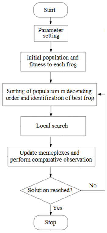
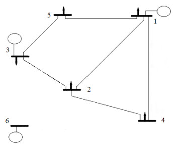
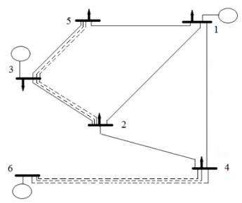
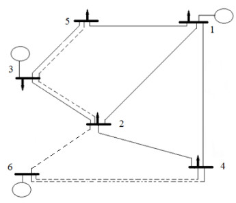
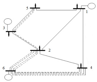
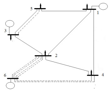
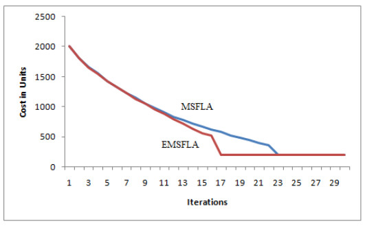
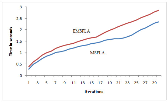
Bio-inspired computing has progressed so far to deal with real-time multi-objective optimization problems. The Transmission expansion planning of the modern electricity grid requires finding the best and optimal routes for electricity transmission from the generation point to the endpoint while satisfying all the power and load constraints. Further, the transmission expansion cost allocation becomes a critical and pragmatic issue in the deregulated electricity industry. The prime objective is to minimize the total investment and expansion costs while considering N-1 contingency. The most optimal transmission expansion planning problem's solution is calculated using the objective function and the constraints. This optimal solution provides the total number and best locations for the candidates. The presented paper details the mathematical modeling of the shuffled frog leap algorithm with various modifications applied to the method to refine the results and finally proposes an enhanced novel approach to solve the transmission expansion planning problem. The proposed algorithm produces the expansion plans based on target-based evolution. The presented algorithm is rigorously tested on the standard Garver dataset and IEEE 24 bus system. The empirical results of the proposed algorithm led to better expansion plans while effectively considering typical electrical constraints along with modern and realistic constraints.
Citation: Smita Shandilya, Ivan Izonin, Shishir Kumar Shandilya, Krishna Kant Singh. Mathematical modelling of bio-inspired frog leap optimization algorithm for transmission expansion planning[J]. Mathematical Biosciences and Engineering, 2022, 19(7): 7232-7247. doi: 10.3934/mbe.2022341
Bio-inspired computing has progressed so far to deal with real-time multi-objective optimization problems. The Transmission expansion planning of the modern electricity grid requires finding the best and optimal routes for electricity transmission from the generation point to the endpoint while satisfying all the power and load constraints. Further, the transmission expansion cost allocation becomes a critical and pragmatic issue in the deregulated electricity industry. The prime objective is to minimize the total investment and expansion costs while considering N-1 contingency. The most optimal transmission expansion planning problem's solution is calculated using the objective function and the constraints. This optimal solution provides the total number and best locations for the candidates. The presented paper details the mathematical modeling of the shuffled frog leap algorithm with various modifications applied to the method to refine the results and finally proposes an enhanced novel approach to solve the transmission expansion planning problem. The proposed algorithm produces the expansion plans based on target-based evolution. The presented algorithm is rigorously tested on the standard Garver dataset and IEEE 24 bus system. The empirical results of the proposed algorithm led to better expansion plans while effectively considering typical electrical constraints along with modern and realistic constraints.

| [1] |
M. A. Attia, M. Arafa, E. A. Sallam, M. M. Fahmy, An enhanced differential evolution algorithm with multi-mutation strategies and self-adapting control parameters, Int. J. Intell. Syst. Appl., 11 (2019), 26-38. https://doi.org/10.5815/ijisa.2019.04.03 doi: 10.5815/ijisa.2019.04.03

|
| [2] |
S. Chakroborty, M. B. Hasan, A proposed technique for solving scenario based multi-period stochastic optimization problems with computer application, Int. J. Math. Sci. Comput., 2 (2016), 12-23. https://doi.org/10.5815/ijmsc.2016.04.02 doi: 10.5815/ijmsc.2016.04.02
|
| [3] | C. W. Lee, S. K. Ng, J. Zhong, F. F. Wu, Transmission expansion planning from past to future, in 2006 IEEE PES Power Systems Conference and Exposition, (2006), 257-265. https://doi.org/10.1109/PSCE.2006.296317 |
| [4] | R. C. G. Teive, A. Hawken, M. A. Laugthon, Knowledge-based system for electrical power networks transmission expansion planning, in 2004 IEEE/PES Transmision and Distribution Conference and Exposition: Latin America, (2004), 435-440. |
| [5] |
R. S. Chanda, P. K. Bhattacharjee, A reliability approach to transmission expansion planning using fuzzy fault-tree model, Electr. Power Syst. Res., 45 (1998), 101-108. https://doi.org/10.1016/S0378-7796(97)01226-1 doi: 10.1016/S0378-7796(97)01226-1
|
| [6] |
A. S. Silva, E. N. Asada, Combined heuristic with fuzzy system to transmission system expansion planning, Electr. Power Syst. Res., 81 (2011), 123-128. https://doi.org/10.1016/j.epsr.2010.07.021 doi: 10.1016/j.epsr.2010.07.021
|
| [7] |
Y. Wang, H. Cheng, C. Wang, Z. Hua, L. Yao, Z. Ma, et al., Pareto optimality-based multi-objective transmission planning considering transmission congestion, Electr. Power Syst. Res., 78 (2008), 1619-1626. https://doi.org/10.1016/j.epsr.2008.02.004 doi: 10.1016/j.epsr.2008.02.004
|
| [8] |
Y. Jin, H. Cheng, J. Yan, L. Zhang, New discrete method for particle swarm optimization and its application in transmission network expansion planning, Electr. Power Syst. Res., 77 (2007), 227-233. https://doi.org/10.1016/j.epsr.2006.02.016 doi: 10.1016/j.epsr.2006.02.016
|
| [9] |
T. S. Chung, K. K. Li, G. J. Chen, J. D. Xie, G. Q. Tang, Multi-objective transmission network planning by a hybrid GA approach with fuzzy decision analysis, Int. J. Electr. Power Energy Syst., 25 (2003), 187-192. https://doi.org/10.1016/S0142-0615(02)00079-0 doi: 10.1016/S0142-0615(02)00079-0
|
| [10] | N. Leeprechanon, P. Limsakul, S. Pothiya, Optimal transmission expansion planning using ant colony optimization, J. Sustainable Energy. Environ., 1 (2010), 71-76. |
| [11] |
S. Jaganathan, C. S. Kumar, S. Palaniswami, Multi objective optimization for transmission network expansion planning using modified bacterial foraging technique, Int. J. Comput. Appl., 9 (2010), 28-34. https://doi.org/10.5120/1364-1839 doi: 10.5120/1364-1839
|
| [12] | J. Contreras, A cooperative game theory approach to transmission planning in power systems, PhD Thesis, University of Castilla-La Mancha, 1997. |
| [13] | M. Eghbal, T. K. Saha, K. N. Hasan, Transmission expansion planning by meta-heuristic techniques: A comparison of Shuffled Frog Leaping Algorithm, PSO and GA, in 2011 IEEE Power and Energy Society General Meeting, (2011), 1-8. |
| [14] |
M. M. Eusuff, K. E. Lansey, Optimization of water distribution network design using the Shuffled Frog Leaping Algorithm, J. Water Resour. Plann. Manage. 129 (2003), 210-225. https://doi.org/10.1061/(ASCE)0733-9496(2003)129:3(210) doi: 10.1061/(ASCE)0733-9496(2003)129:3(210)
|
| [15] | S. Liong, M. Atiquzzaman, Optimal design of water distribution network using shuffled complex evolution, J. Inst. Eng., 2004. |
| [16] |
M. Eusuff, K. Lansey, F. Pasha, Shuffled frog-leaping algorithm: a memetic meta-heuristic for discrete optimization, Eng. Optim., 38 (2006), 129-154. https://doi.org/10.1080/03052150500384759 doi: 10.1080/03052150500384759
|
| [17] |
F. H. Eid, M. A. Kamilah, Adjustive reciprocal whale optimization algorithm for wrapper attribute selection and classification, Int. J. Image Graphics Signal Processing, 11 (2019), 18-26. https://doi.org/10.5815/ijigsp.2019.03.03 doi: 10.5815/ijigsp.2019.03.03
|
| [18] |
P. Dutta, M. Majumder, A. Kumar, Parametric optimization of liquid flow process by ANOVA optimized DE, PSO & GA algorithms, Int. J. Image Graphics Signal Processing, 11 (2021), 14-24. https://doi.org/10.5815/ijem.2021.05.02 doi: 10.5815/ijem.2021.05.02
|
| [19] | B. M. Sreedhara, G. Kuntoji, S. Mandal, Application of particle swarm based neural network to predict scour depth around the bridge pier, Int. J. Intell. Syst. Appl., 11 (2019), 38-47. |
| [20] | T. Saw, P. H. Myint, Feature selection to classify healthcare data using wrapper method with PSO search, Int. J. Inf. Technol. Comput. Sci., 11 (2019), 31-37. |
| [21] | O. Bisikalo, D. Chernenko, O. Danylchuk, V. Kovtun, V. Romanenko, Information technology for TTF optimization of an information system for critical use that operates in aggressive Cyber-physical space, in 2020 IEEE International Conference on Problems of Infocommunications, Science and Technology, (2020), 323-329. https://doi.org/10.1109/PICST51311.2020.9467997 |
| [22] | N. Pasyeka, H. Mykhailyshyn, M. Pasyeka, Development algorithmic model for optimization of distributed fault-tolerant web-systems, in 2018 International Scientific-Practical Conference Problems of Infocommunications. Science and Technology, (2018), 663-669. |
| [23] | A Hussain, I Ahmad, Development a new crossover scheme for traveling salesman problem by aid of genetic algorithm, Int. J. Intell. Syst. Appl., 11 (2019), 46-52. |
| [24] |
P. S. D. Nutheti, N. Hasyagar, R. Shettar, G. Shankr, V. Umadevi, Ferrer diagram based partitioning technique to decision tree using genetic algorithm, Int. J. Math. Sci. Comput., 6 (2020), 25-32. https://doi.org/10.5815/ijmsc.2020.01.03 doi: 10.5815/ijmsc.2020.01.03
|
| [25] | M. P. Aghababa, M. E. Akbari, A. M. Shotorbani, R. M. Shotorbani, Application of modified shuffled frog leaping algorithm for robot optimal controller design, Int. J. Sci. Eng. Res., 2 (2011), 6. |
| [26] |
J. M. Ling, A. S. Khuong, Modified shuffled frog-leaping algorithm on optimal planning for a stand-alone photovoltaic system, Appl. Mech. Mater., 145 (2011), 574-578. https://doi.org/10.4028/www.scientific.net/AMM.145.574 doi: 10.4028/www.scientific.net/AMM.145.574
|
| [27] | M. Farahani, S. B. Movahhed, S. F. Ghaderi, A hybrid meta-heuristic optimization algorithm based on SFLA, 2 nd Int. Confer. Eng. Optim., (2010), 1-8. |
| [28] | R. Bayat, H. Ahmadi, Artificial intelligence SVC based control of two machine transmission system, Int. J. Intell. Syst. Appl., 5 (2013), 1-8. |
| [29] | R. Malviya, R. K. Saxena, Modified approach for harmonic reduction in transmission system using 48-pulse UPFC employing series Zig-Zag primary and Y-Y secondary transformer, Int. J. Intell. Syst. Appl., 5 (2013), 70-79. |
| [30] |
L. Garver, Transmission network estimation using linear programming, IEEE Trans. Power Apparatus Syst., 89 (1970), 1688-1697. https://doi.org/10.1109/TPAS.1970.292825 doi: 10.1109/TPAS.1970.292825
|
| [31] |
Z. Hu, M. Ivashchenko, L. Lyushenko, D. Klyushnyk, Artificial neural network training criterion formulation using error continuous domain, Int.J. Modern Edu. Comput. Sci., 13 (2021), 13-22. https://doi.org/10.5815/ijmecs.2021.03.02 doi: 10.5815/ijmecs.2021.03.02
|
| [32] |
Z. Hu, I. A. Tereykovskiy, L. O. Tereykovska, V. V. Pogorelov, Determination of structural parameters of multilayer perceptron designed to estimate parameters of technical systems, Int. J. Intell. Syst. Appl., 9 (2017), 57-62. https://doi.org/10.5815/ijisa.2017.10.07 doi: 10.5815/ijisa.2017.10.07
|

Figures(12) / Tables(2)

Smita Shandilya, Ivan Izonin, Shishir Kumar Shandilya, Krishna Kant Singh. Mathematical modelling of bio-inspired frog leap optimization algorithm for transmission expansion planning[J]. Mathematical Biosciences and Engineering, 2022, 19(7): 7232-7247. doi: 10.3934/mbe.2022341


 DownLoad: