Epidemiology of coronavirus disease 2019 (COVID-19) in Japan during the first and second waves

Ryo Kinoshita; Sung-mok Jung; Tetsuro Kobayashi; Andrei R. Akhmetzhanov; Hiroshi Nishiura; Ryo Kinoshita; Sung-mok Jung; Tetsuro Kobayashi; Andrei R. Akhmetzhanov; Hiroshi Nishiura

doi:10.3934/mbe.2022284

Mathematical Biosciences and Engineering

2022, Volume 19, Issue 6: 6088-6101. doi: 10.3934/mbe.2022284

Previous Article Next Article

Research article Special Issues

Epidemiology of coronavirus disease 2019 (COVID-19) in Japan during the first and second waves

1.
School of Public Health, Kyoto University, Kyoto, Japan
2.
National Institute of Infectious Diseases, Center of Surveillance Immunization and Epidemiologic Research, Tokyo, Japan
3.
Graduate School of Medicine, Hokkaido University, Sapporo, Japan
4.
College of Public Health, National Taiwan University, Taipei, Taiwan

Received: 10 January 2022 Revised: 28 March 2022 Accepted: 28 March 2022 Published: 13 April 2022

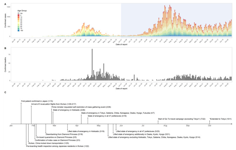
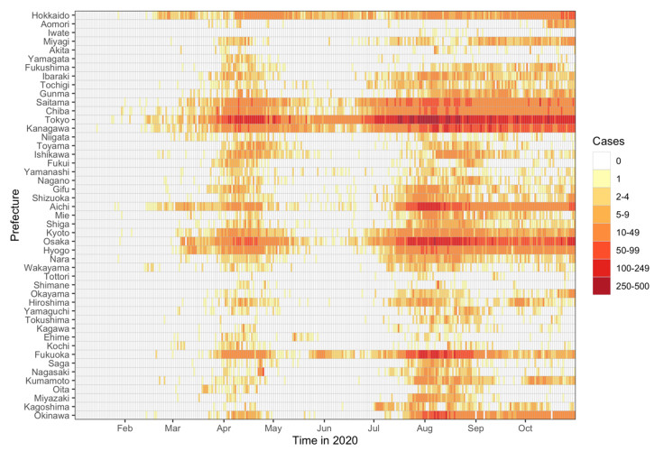
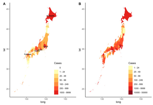
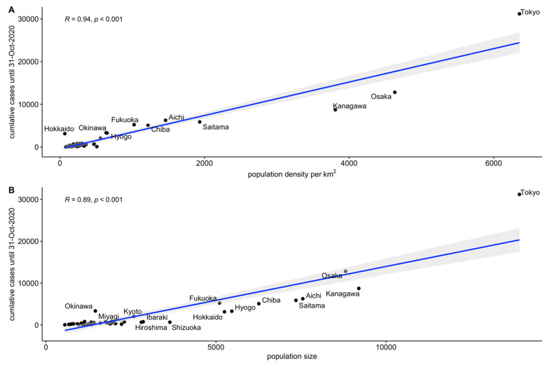
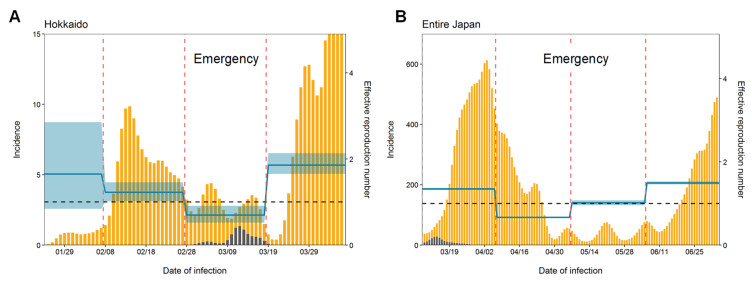
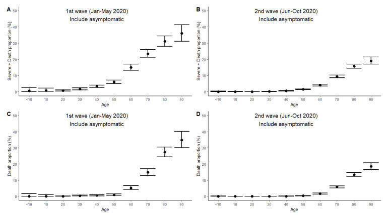
Following the emergence and worldwide spread of coronavirus disease 2019 (COVID-19), each country has attempted to control the disease in different ways. The first patient with COVID-19 in Japan was diagnosed on 15 January 2020, and until 31 October 2020, the epidemic was characterized by two large waves. To prevent the first wave, the Japanese government imposed several control measures such as advising the public to avoid the 3Cs (closed spaces with poor ventilation, crowded places with many people nearby, and close-contact settings such as close-range conversations) and implementation of "cluster buster" strategies. After a major epidemic occurred in April 2020 (the first wave), Japan asked its citizens to limit their numbers of physical contacts and announced a non-legally binding state of emergency. Following a drop in the number of diagnosed cases, the state of emergency was gradually relaxed and then lifted in all prefectures of Japan by 25 May 2020. However, the development of another major epidemic (the second wave) could not be prevented because of continued chains of transmission, especially in urban locations. The present study aimed to descriptively examine propagation of the COVID-19 epidemic in Japan with respect to time, age, space, and interventions implemented during the first and second waves. Using publicly available data, we calculated the effective reproduction number and its associations with the timing of measures imposed to suppress transmission. Finally, we crudely calculated the proportions of severe and fatal COVID-19 cases during the first and second waves. Our analysis identified key characteristics of COVID-19, including density dependence and also the age dependence in the risk of severe outcomes. We also identified that the effective reproduction number during the state of emergency was maintained below the value of 1 during the first wave.
- SARS-CoV-2,
- COVID-19,
- Japan,
- descriptive epidemiology
Citation: Ryo Kinoshita, Sung-mok Jung, Tetsuro Kobayashi, Andrei R. Akhmetzhanov, Hiroshi Nishiura. Epidemiology of coronavirus disease 2019 (COVID-19) in Japan during the first and second waves[J]. Mathematical Biosciences and Engineering, 2022, 19(6): 6088-6101. doi: 10.3934/mbe.2022284

Related Papers:

Abstract

Following the emergence and worldwide spread of coronavirus disease 2019 (COVID-19), each country has attempted to control the disease in different ways. The first patient with COVID-19 in Japan was diagnosed on 15 January 2020, and until 31 October 2020, the epidemic was characterized by two large waves. To prevent the first wave, the Japanese government imposed several control measures such as advising the public to avoid the 3Cs (closed spaces with poor ventilation, crowded places with many people nearby, and close-contact settings such as close-range conversations) and implementation of "cluster buster" strategies. After a major epidemic occurred in April 2020 (the first wave), Japan asked its citizens to limit their numbers of physical contacts and announced a non-legally binding state of emergency. Following a drop in the number of diagnosed cases, the state of emergency was gradually relaxed and then lifted in all prefectures of Japan by 25 May 2020. However, the development of another major epidemic (the second wave) could not be prevented because of continued chains of transmission, especially in urban locations. The present study aimed to descriptively examine propagation of the COVID-19 epidemic in Japan with respect to time, age, space, and interventions implemented during the first and second waves. Using publicly available data, we calculated the effective reproduction number and its associations with the timing of measures imposed to suppress transmission. Finally, we crudely calculated the proportions of severe and fatal COVID-19 cases during the first and second waves. Our analysis identified key characteristics of COVID-19, including density dependence and also the age dependence in the risk of severe outcomes. We also identified that the effective reproduction number during the state of emergency was maintained below the value of 1 during the first wave.

References

[1]	Q. Li, X. Guan X, P. Wu, X. Wang, L. Zhou, Y. Tong, et al., Early transmission dynamics in Wuhan, China, of novel coronavirus-infected pneumonia, N. Engl. J. Med., 382 (2020), 1199-1207. https://doi.org/10.1056/NEJMoa2001316 doi: 10.1056/NEJMoa2001316
[2]	I. I. Bogoch, A. Watts, A. Thomas-Bachli, C, Huber, M. U. Kraemer, K. Khan, Pneumonia of unknown aetiology in Wuhan, China: Potential for international spread via commercial air travel, J. Travel Med., 27 (2020). https://doi.org/10.1093/jtm/taaa008 doi: 10.1093/jtm/taaa008
[3]	H. Nishiura, T. Kobayashi, Y. Yang, K. Hayashi, T. Miyama, R. Kinoshita, et al., The rate of underascertainment of novel coronavirus (2019-nCoV) infection: Estimation using Japanese passengers data on evacuation flights, J. Clin. Med., 9 (2020), 419. https://doi.org/10.3390/jcm9020419 doi: 10.3390/jcm9020419
[4]	K. Mizumoto, K. Kagaya, A. Zarebski, G. Chowell, Estimating the asymptomatic proportion of coronavirus disease 2019 (COVID-19) cases on board the Diamond Princess cruise ship, Yokohama, Japan, 2020, Eurosurveillance, 25 (2020), 2000180. https://doi.org/10.2807/1560-7917.ES.2020.25.10.2000180 doi: 10.2807/1560-7917.ES.2020.25.10.2000180
[5]	T. Sekizuka, K. Itokawa, M. Hashino, T. Kawano-Sugaya, R. Tanaka, L. Yatsu, et al., A genome epidemiological study of SARS-CoV-2 introduction into Japan, MSphere, 5 (2020), e00786-20. https://doi.org/10.1128/mSphere.00786-20 doi: 10.1128/mSphere.00786-20
[6]	Y. Furuse, Y. K. Ko, M. Saito, Y. Shobugawa, K. Jindai, T. Saito, et al., Epidemiology of COVID-19 outbreak in Japan, January-March 2020, Jpn. J. Infect. Dis., 73 (2020), 391-393. https://doi.org/10.7883/yoken.JJID.2020.271 doi: 10.7883/yoken.JJID.2020.271
[7]	H. Oshitani, Cluster-based approach to coronavirus disease 2019 (COVID-19) response in Japan, from February to April 2020, Jpn. J. Infect. Dis., 73 (2020), 491-493. https://doi.org/0.7883/yoken.JJID.2020.363
[8]	Y. Furuse, E. Sando, N. Tsuchiya, R. Miyahara, I. Yasuda, Y. K. Ko, et al., Clusters of coronavirus disease in communities, Japan, January-April 2020, Emerg. Infect. Dis., 26 (2020), 2176-2179. https://doi.org/10.3201/eid2609.202272 doi: 10.3201/eid2609.202272
[9]	H. Nishiura, H. Oshitani, T. Kobayashi, T. Saito, T. Sunagawa, T. Matsui, et al., Closed environments facilitate secondary transmission of coronavirus disease 2019 (COVID-19), medRxiv, 2020. https://doi.org/https://doi.org/10.1101/2020.02.28.20029272. doi: 10.1101/2020.02.28.20029272
[10]	A. Endo, S. Abbott, A.J. Kucharski, S. Funk, Estimating the overdispersion in COVID-19 transmission using outbreak sizes outside China, Wellcome Open Res., 5 (2020), 67. https://doi.org/10.12688/wellcomeopenres.15842.3 doi: 10.12688/wellcomeopenres.15842.3
[11]	A. Anzai, H. Nishiura, "Go To Travel" campaign and travel-associated coronavirus disease 2019 cases: A descriptive analysis, July-August 2020, J. Clin. Med., 10 (2021), 398. https://doi.org/10.3390/jcm10030398 doi: 10.3390/jcm10030398
[12]	Open data (COVID-19), Ministry of Health Labour and Welfare of Japan, 2021. Available from: https://www.mhlw.go.jp/stf/covid-19/open-data.html.
[13]	S. M. Jung, A. R. Akhmetzhanov, K. Hayashi, N. M. Linton, Y. Yang, B. Yuan, et al., Real-time estimation of the risk of death from novel coronavirus (COVID-19) infection: Inference using exported cases, J. Clin. Med., 9 (2020), 523. https://doi.org/10.3390/jcm9020523 doi: 10.3390/jcm9020523
[14]	S. M. Jung, A. Endo, A. R. Akhmetzhanov, H. Nishiura, Predicting the effective reproduction number of COVID-19: Inference using human mobility, temperature, and risk awareness, Int. J. Infect. Dis., 113 (2020), 47-54. https://doi.org/10.1016/j.ijid.2021.10.007 doi: 10.1016/j.ijid.2021.10.007
[15]	M. Höhle, A. Riebler, The R package 'surveillance', 2005. Available from: https://cran.r-project.org/web/packages/surveillance/index.html.
[16]	N. M. Linton, T. Kobayashi, Y. Yang, K. Hayashi, A. R. Akhmetzhanov, S. M. Jung, et al., Incubation period and other epidemiological characteristics of 2019 novel coronavirus infections with right truncation: A statistical analysis of publicly available case data, J. Clin. Med., 9 (2020), 538. https://doi.org/10.3390/jcm9020538. doi: 10.3390/jcm9020538
[17]	H. Nishiura, N. M. Linton, A. R. Akhmetzhanov, Serial interval of novel coronavirus (COVID-19) infections, Int. J. Infect. Dis., 93 (2020), 284-286. https://doi.org/10.1016/j.ijid.2020.02.060 doi: 10.1016/j.ijid.2020.02.060
[18]	T. K. Boehmer, J. DeVies, E. Caruso, K. L. van Santen, S. Tang, C. L. Black, et al., Changing Age Distribution of the COVID-19 Pandemic-United States, May-August 2020, MMWR Morb. Mortal. Wkly. Rep., 69 (2020), 1404-1409. https://doi.org/10.15585/mmwr.mm6939e1 doi: 10.15585/mmwr.mm6939e1
[19]	A. R. Akhmetzhanov, K. Mizumoto, S. M. Jung, N. M. Linton, R. Omori, H. Nishiura, Estimation of the actual incidence of coronavirus disease (COVID-19) in emergent hotspots: The example of Hokkaido, Japan during February-March 2020, J. Clin. Med., 10 (2021), 2392. https://doi.org/10.3390/jcm10112392 doi: 10.3390/jcm10112392
[20]	COVID-19 Google community mobility reports, Google, Available from: https://www.google.com/covid19/mobility/.
[21]	P. Wilmes, J. Zimmer, J. Schulz, F. Glod, L. Veiber, L. Mombaerts, et al., SARS-CoV-2 transmission risk from asymptomatic carriers: Results from a mass screening programme in Luxembourg, Lancet Reg. Health Eur., 4 (2021), 100056. https://doi.org/10.1016/j.lanepe.2021.100056 doi: 10.1016/j.lanepe.2021.100056
[22]	R. Omori, K. Mizumoto, H. Nishiura, Ascertainment rate of novel coronavirus disease (COVID-19) in Japan, Int. J. Infect. Dis., 96 (2020), 673-675. https://doi.org/10.1016/j.ijid.2020.04.080 doi: 10.1016/j.ijid.2020.04.080
[23]	T. Kawashima, S. Nomura, Y. Tanoue, D. Yoneoka, A. Eguchi, C.F.S. Ng, et al., Excess all-cause deaths during coronavirus disease pandemic, Japan, January-May 2020, Emerg. Infect. Dis., 27 (2021), 789-795. https://doi.org/10.3201/eid2703.203925. doi: 10.3201/eid2703.203925
[24]	T. Yoshiyama, Y. Saito, K. Masuda, Y. Nakanishi, Y. Kido, K. Uchimura, et al., Prevalence of SARS-CoV-2-specific antibodies, Japan, June 2020, Emerg. Infect. Dis., 27 (2021), 628-631. https://doi.org/10.3201/eid2702.204088 doi: 10.3201/eid2702.204088

mbe-19-06-284-supplementary.pdf

Reader Comments

Your name:*

Email:*
© 2022 the Author(s), licensee AIMS Press. This is an open access article distributed under the terms of the Creative Commons Attribution License (http://creativecommons.org/licenses/by/4.0)