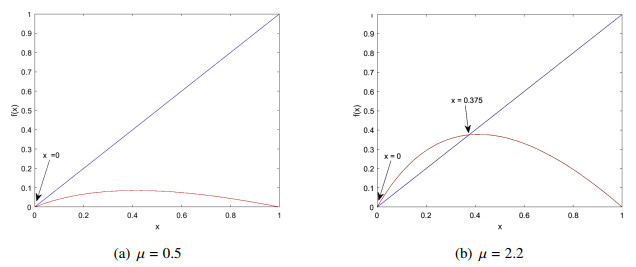
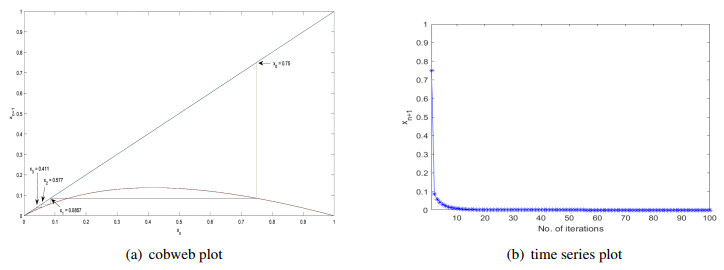
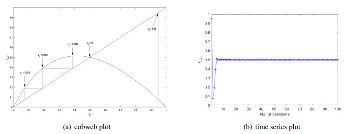
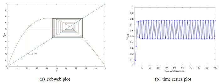
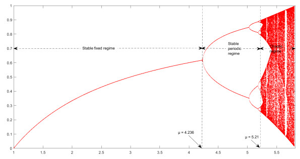
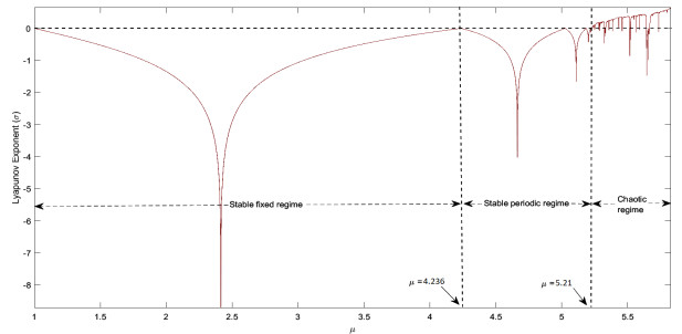
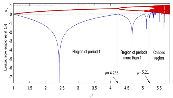
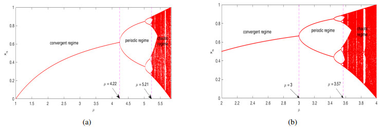
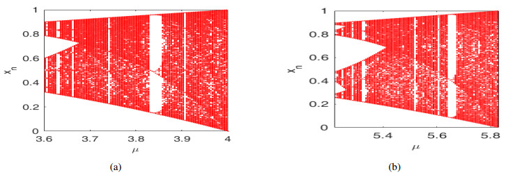
In this paper, a novel one dimensional chaotic map $ K(x) = \frac{\mu x(1\, -x)}{1+ x} $, $ x\in [0, 1], \mu > 0 $ is proposed. Some dynamical properties including fixed points, attracting points, repelling points, stability and chaotic behavior of this map are analyzed. To prove the main result, various dynamical techniques like cobweb representation, bifurcation diagrams, maximal Lyapunov exponent, and time series analysis are adopted. Further, the entropy and probability distribution of this newly introduced map are computed which are compared with traditional one-dimensional chaotic logistic map. Moreover, with the help of bifurcation diagrams, we prove that the range of stability and chaos of this map is larger than that of existing one dimensional logistic map. Therefore, this map might be used to achieve better results in all the fields where logistic map has been used so far.
Citation: Amit Kumar, Jehad Alzabut, Sudesh Kumari, Mamta Rani, Renu Chugh. Dynamical properties of a novel one dimensional chaotic map[J]. Mathematical Biosciences and Engineering, 2022, 19(3): 2489-2505. doi: 10.3934/mbe.2022115
In this paper, a novel one dimensional chaotic map $ K(x) = \frac{\mu x(1\, -x)}{1+ x} $, $ x\in [0, 1], \mu > 0 $ is proposed. Some dynamical properties including fixed points, attracting points, repelling points, stability and chaotic behavior of this map are analyzed. To prove the main result, various dynamical techniques like cobweb representation, bifurcation diagrams, maximal Lyapunov exponent, and time series analysis are adopted. Further, the entropy and probability distribution of this newly introduced map are computed which are compared with traditional one-dimensional chaotic logistic map. Moreover, with the help of bifurcation diagrams, we prove that the range of stability and chaos of this map is larger than that of existing one dimensional logistic map. Therefore, this map might be used to achieve better results in all the fields where logistic map has been used so far.

| [1] | J. Gleick, Chaos: Making a New Science, Viking Books, New York, 1997. |
| [2] | I. Prigogine, I. Stengers, A. Toffler, Order Out of Chaos: Man's New Dialogue with Nature, Bantam Books, New York, 1984. |
| [3] | E. Ott, Chaos in Dynamical Systems, Cambridge University Press, Cambridge, 2002. |
| [4] |
E. N. Lorenz, Deterministic nonperiodic flow, J. Atmos Sci., 20 (1963), 130–141. https://doi.org/10.1175/1520-0469(1963)020<0130:DNF>2.0.CO;2. doi: 10.1175/1520-0469(1963)020<0130:DNF>2.0.CO;2

|
| [5] |
R. M. May, Simple mathematical models with very complicated dynamics, Nature, 261 (1976), 459–465. https://doi.org/10.1038/261459a0. doi: 10.1038/261459a0
|
| [6] | M. F. Barnsley, Fractals Everywhere, 2$^nd$ edition, Revised with the assistance of and a foreword by Hawley Rising, Academic Press Professional, Boston, 1993. |
| [7] |
F. M. Atay, J. Jost, A. Wende, Delays, connection topology, and synchronization of coupled chaotic maps, Phys. Rev. Lett., 92 (2004), 1–5. https://doi.org/10.1103/PhysRevLett.92.144101. doi: 10.1103/PhysRevLett.92.144101
|
| [8] |
K. M. Cuomo, A. V. Oppenheim, Circuit implementation of synchronized chaos with applications to communications, Phys. Rev. Lett., 71 (1993), 65–68. https://doi.org/10.1103/PhysRevLett.71.65. doi: 10.1103/PhysRevLett.71.65
|
| [9] |
I. Klioutchnikova, M. Sigovaa, N. Beizerov, Chaos Theory in Finance, Procedia Comput. Sci., 119 (2017), 368–375. https://doi.org/10.1016/j.procs.2017.11.196. doi: 10.1016/j.procs.2017.11.196
|
| [10] | Y. Sun, G. Qi, Z. Wang, B. J. Y. Wyk, Y. Haman, Chaotic particle swarm optimization, in Proceedings of the 11th Annual Conference Companion on Genetic and Evolutionary Computation Conference, (2009), 12–14. |
| [11] |
S. Behnia, A. Akhshani, H. Mahmodi, A. Akhavan, A novel algorithm for image encryption based on mixture of chaotic maps, Chaos Soliton Fract., 35 (2008), 408–419. https://doi.org/10.1016/j.chaos.2006.05.011. doi: 10.1016/j.chaos.2006.05.011
|
| [12] |
N. K. Pareek, V. Patidar, K. K. Sud, Image encryption using chaotic logistic map, Img. Vis. Comput., 24 (2006), 926–934. https://doi.org/10.1016/j.imavis.2006.02.021. doi: 10.1016/j.imavis.2006.02.021
|
| [13] | X. Y. Wang, Synchronization of Chaos Systems and their Application in Secure Communication, Science Press, Beijing, 2012. |
| [14] | K. M. U. Maheswari, R. Kundu, H. Saxena, Pseudo random number generators algorithms and applications, Int. J. Pure Appl. Math., 118 (2018), 331–336. |
| [15] |
L. Wang, H. Cheng, Pseudo-random number generator based on logistic chaotic system, Entropy, 21 (2019), 1–12. https://doi.org/10.3390/e21100960. doi: 10.3390/e21100960
|
| [16] |
J. Lü, X. Yu, G. Chen, Chaos synchronization of general complex dynamical networks, Phys. A, 334 (2004), 281–302. https://doi.org/10.1016/j.physa.2003.10.052. doi: 10.1016/j.physa.2003.10.052
|
| [17] |
L. Chen, K. Aihara, Chaotic simulated annealing by a neural network model with transient chaos, Neural Networks, 8 (1995), 915–930. https://doi.org/10.1016/0893-6080(95)00033-V. doi: 10.1016/0893-6080(95)00033-V
|
| [18] |
S. Kumari, R. Chugh, A novel four-step feedback procedure for rapid control of chaotic behavior of the logistic map and unstable traffic on the road, Chaos: Interdiscip. J. Nonlinear Sci., 30 (2020), 123115. doi: https://doi.org/10.1063/5.0022212. doi: 10.1063/5.0022212
|
| [19] | S. Strogatz, Nonlinear Dynamics and Chaos: With Applications to Physics, Biology, Chemistry and Engineering, AIP Publishing, 2001. |
| [20] | R. L. Devaney, An Introduction to Chaotic Dynamical Systems, 2$^nd$ edition, Westview Press, USA, 2003. |
| [21] |
M. Henon, A two-dimensional mapping with a strange attractor, Math Phys., 50 (1976), 69–77. https://doi.org/10.1007/BF01608556. doi: 10.1007/BF01608556
|
| [22] | K. Kaneko, Theory and Application of Coupled Map Lattices, John Wiley and Sons, New York, 1993. |
| [23] |
S. J. Cang, Z. H. Wang, Z. Q. Chen, H. Y. Jia, Analytical and numerical investigation of a new Lorenz-like chaotic attractor with compound structures, Nonlinear Dyn., 75 (2014), 745–760. https://doi.org/10.1007/s11071-013-1101-7. doi: 10.1007/s11071-013-1101-7
|
| [24] |
D. Lambi\'c, A new discrete-space chaotic map based on the multiplication of integer numbers and its application in S-box design, Nonlinear Dyn., 100 (2020), 699–711. https://doi.org/10.1007/s11071-020-05503-y. doi: 10.1007/s11071-020-05503-y
|
| [25] |
S. Kumari, R. Chugh, R. Miculescu, On the complex and chaotic dynamics of standard logistic sine square map, An. Univ. "Ovidius" Constanta - Ser.: Mat., 29 (2021), 201–227. https://doi.org/10.2478/auom-2021-0041. doi: 10.2478/auom-2021-0041
|
| [26] |
L. Liu, S. Miao, A new simple one-dimensional chaotic map and its application for image encryption, Multimedia Tools Appl., 77 (2018), 21445–21462. https://doi.org/10.1007/s11042-017-5594-9. doi: 10.1007/s11042-017-5594-9
|
| [27] |
X. Zhang, Y. Cao, A novel chaotic map and an improved chaos-based image encryption scheme, Sci. World J., 2014 (2014). https://doi.org/10.1155/2014/713541. doi: 10.1155/2014/713541
|
| [28] |
P. Verhulst, The law of population growth, Nouvelles Memories de lÀcadè mie Royale des Sciences et Belles-Lettres de Bruxelles, 18 (1845), 14–54. https://doi.org/10.3406/minf.1845.1813. doi: 10.3406/minf.1845.1813
|
| [29] | R. A. Holmgren, A First Course in Discrete Dynamical Systems, Springer-Verlag, New York, 1996. https://doi.org/10.1007/978-1-4419-8732-7. |
| [30] |
Ashish, J. Cao, R. Chugh, Chaotic behavior of logistic map in superior orbit and an improved chaos-based traffic control model, Nonlinear Dyn., 94 (2018), 959–975. https://doi.org/10.1007/s11071-018-4403-y. doi: 10.1007/s11071-018-4403-y
|
| [31] |
R. Chugh, M. Rani, Ashish, On the convergence of logistic map in noor orbit, Int. J. Comput. Appl., 43 (2012), 0975–8887. https://doi.org/10.5120/6200-8739. doi: 10.5120/6200-8739
|
| [32] | S. Kumari, R. Chugh, A new experiment with the convergence and stability of logistic map via SP orbit, Int. J. Appl. Eng. Res., 14 (2019), 797–801. https://www.ripublication.com. |
| [33] |
S. Kumari, R. Chugh, A. Nandal, Bifurcation analysis of logistic map using four step feedback procedure, Int. J. Eng. Adv. Technol., 9 (2019), 704–707. https://doi.org/10.35940/ijeat.F9166.109119. doi: 10.35940/ijeat.F9166.109119
|
| [34] |
M. Rani, R. Agarwal, A new experimental approach to study the stability of logistic map, Chaos Solitons Fract., 41 (2009), 2062–2066. https://doi.org/10.1016/j.chaos.2008.08.022. doi: 10.1016/j.chaos.2008.08.022
|
| [35] | M. Rani, S. Goel, An experimental approach to study the logistic map in I-superior orbit, Chaos Complexity Lett., 5 (2011), 95–102. |
| [36] |
M. T. Rosenstein, J. J. Collins, C. J. D. Luca, A practical method for calculating largest Lyapunov exponents from small data sets, Phys. D, 65 (1993), 117–134. https://doi.org/10.1016/0167-2789(93)90009-P. doi: 10.1016/0167-2789(93)90009-P
|
| [37] |
A. Wolf, J. B. Swift, H. L. Swinney, J. A. Vastano, Determining Lyapunov exponents from a time series, Phys. D, 16 (1985), 285–317. https://doi.org/10.1016/0167-2789(85)90011-9. doi: 10.1016/0167-2789(85)90011-9
|
| [38] |
A. Balestrino, A. Caiti, E. Crisostomi, Generalized entropy of curves for the analysis and classification of dynamical systems, Entropy, 11 (2009), 249–270. https://doi.org/10.3390/e11020249. doi: 10.3390/e11020249
|
| [39] | A. Balestrino, A. Caiti, E. Crisostomi, A classification of nonlinear systems: An entropy based approach, Chem. Eng. Trans., 11 (2007), 119–124. |
| [40] |
A. Balestrino, A. Caiti, E. Crisostomi, Entropy of curves for nonlinear systems classification, IFAC Proc. Vol., 40 (2007), 72–77. https://doi.org/10.3182/20070822-3-ZA-2920.00012. doi: 10.3182/20070822-3-ZA-2920.00012
|
| [41] |
C. E. Shannon, A mathematical theory of communication, Bell Syst. Tech. J., 27 (1948), 379–423. https://doi.org/10.1002/j.1538-7305.1948.tb01338.x. doi: 10.1002/j.1538-7305.1948.tb01338.x
|
| [42] |
S. Behnia, A. Akhshani, S. Ahadpour, H. Mahmodi, A. Akhavan, A fast chaotic encryption scheme based on piecewise nonlinear chaotic maps, Phys. Lett. A, 366 (2007), 391–396. https://doi.org/10.1016/j.physleta.2007.01.081. doi: 10.1016/j.physleta.2007.01.081
|
| [43] |
E. Fatemi-Behbahani, K. Ansari-Asl, E. Farshidi, A new approach to analysis and design of chaos-based random number generators using algorithmic converter, Circuits Syst. Signal Process., 35 (2016), 3830–3846. https://doi.org/10.1007/s00034-016-0248-0. doi: 10.1007/s00034-016-0248-0
|
| [44] |
L. Liu, S. Miao, H. Hu, Y. Deng, Pseudo-random bit generator based on non-stationary logistic maps, IET Inf. Secur., 10 (2016), 87–94. https://doi.org/10.1049/iet-ifs.2014.0192. doi: 10.1049/iet-ifs.2014.0192
|
| [45] |
A. Kanso, N. Smaoui, Logistic chaotic maps for binary numbers generations, Chaos, Solitons Fractals, 40 (2009), 2557–2568. https://doi.org/10.1016/j.chaos.2007.10.049. doi: 10.1016/j.chaos.2007.10.049
|
| [46] |
C. Liu, L. Ding, Q. Ding, Research about the characteristics of chaotic systems based on multi-scale entropy, Entropy, 21 (2019), 663. https://doi.org/10.3390/e21070663. doi: 10.3390/e21070663
|
| [47] |
L. Wang, H. Cheng, Pseudo-random number generator based on logistic chaotic system, Entropy, 21 (2019), 960. https://doi.org/10.3390/e21100960. doi: 10.3390/e21100960
|
| [48] | J. Fridrich, Image encryption based on chaotic maps, in Proceedings of IEEE International Conference on Systems, Man and Cybernetics(ICSMC'97), 2 (1997), 1105–1110. |
| [49] | S. Li, Q. Li, W. Li, X. Mou, Y. Cai, Statistical properties of digital piecewise linear chaotic maps and their roles in cryptography and pseudo-random coding, in IMA International Conference on Cryptography and Coding, 2260 (2001), 205–221. https: //doi.org/10.1007/3-540-45325-3_19. |
| [50] |
L. M. Pecora, T. L. Carroll, Synchronization in chaotic systems, Phys. Rev. Lett., 64 (1990), 821–824. https://doi.org/10.1103/PhysRevLett.64.821. doi: 10.1103/PhysRevLett.64.821
|
Figures(12) / Tables(2)

Amit Kumar, Jehad Alzabut, Sudesh Kumari, Mamta Rani, Renu Chugh. Dynamical properties of a novel one dimensional chaotic map[J]. Mathematical Biosciences and Engineering, 2022, 19(3): 2489-2505. doi: 10.3934/mbe.2022115


 DownLoad: