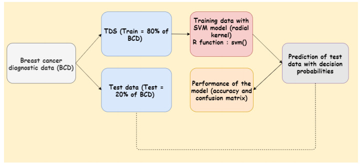
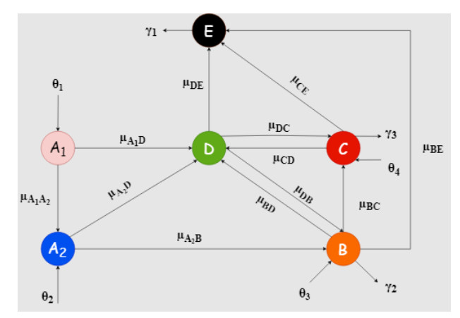
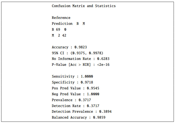
Breast cancer is the most common type of cancer in women. Its mortality rate is high due to late detection and cardiotoxic effects of chemotherapy. In this work, we used the Support Vector Machine (SVM) method to classify tumors and proposed a new mathematical model of the patient dynamics of the breast cancer population. Numerical simulations were performed to study the behavior of the solutions around the equilibrium point. The findings revealed that the equilibrium point is stable regardless of the initial conditions. Moreover, this study will help public health decision-making as the results can be used to minimize the number of cardiotoxic patients and increase the number of recovered patients after chemotherapy.
Citation: Cyrille Agossou, Mintodê Nicodème Atchadé, Aliou Moussa Djibril, Svetlana Vladimirovna Kurisheva. Mathematical modeling and machine learning for public health decision-making: the case of breast cancer in Benin[J]. Mathematical Biosciences and Engineering, 2022, 19(2): 1697-1720. doi: 10.3934/mbe.2022080
Breast cancer is the most common type of cancer in women. Its mortality rate is high due to late detection and cardiotoxic effects of chemotherapy. In this work, we used the Support Vector Machine (SVM) method to classify tumors and proposed a new mathematical model of the patient dynamics of the breast cancer population. Numerical simulations were performed to study the behavior of the solutions around the equilibrium point. The findings revealed that the equilibrium point is stable regardless of the initial conditions. Moreover, this study will help public health decision-making as the results can be used to minimize the number of cardiotoxic patients and increase the number of recovered patients after chemotherapy.

| [1] | Qu'est-ce que le cancer du sein, 2020, available from: https://www.lillyoncologie.fr/cancer-du-sein/definition, (accessed on: 21-07-2021). |
| [2] |
M. Ly, M. Antoine, F. André, P. Callard, J. F. Bernaudin, D. A. Diallo, Le cancer du sein chez la femme de l'Afrique sub-saharienne : état actuel des connaissances, Bulletin du Cancer, 98, (2011), 797–806. doi: 10.1684/bdc.2011.1392. doi: 10.1684/bdc.2011.1392

|
| [3] | Breast cancer, 2021, available from: https://www.who.int/news-room/fact-sheets/detail/breast-cancer, (accessed on: 10-06-2021). |
| [4] |
N. Azamjah, Y. Soltan-Zadeh, F. Zayeri, Global trend of breast cancer mortality rate: a 25-year study, Asian Pac. J. Cancer Prev., 20, (2019), 2015–2020. doi: 10.31557/APJCP.2019.20.7.2015 doi: 10.31557/APJCP.2019.20.7.2015
|
| [5] |
D. G. Gbessi, I. Lawani, C. Tawo-Nounagnon, F. Dossou, Y. Souaïbou, D. Mehinto, et al., Management of Breast Cancer in Visceral Surgery of CNHU-HKM of Cotonou in Benin, Surg. Sci., 07 (2016), 170–176. doi: 10.4236/ss.2016.73022. doi: 10.4236/ss.2016.73022
|
| [6] | G. Deloeuvre, Comprendre le cancer, 2018, available from: https://urlz.fr/guSV, (accessed on: 10-06-2021). |
| [7] | Cancers du sein: les facteurs de risque, 2021, available from: https://www.fondation-arc.org/cancer/cancer-sein/facteurs-risque-cancer, (accessed on: 20-06-2021). |
| [8] | X. Gruffat, Cancer du sein : Résumé sur le cancer du sein, 2021, available from: https://www.creapharma.ch/cancer-du-sein.htm, (accessed on: 10-03-2021). |
| [9] | Cancer du sein, 2019, available from: https://www.cancer-environnement.fr/144-Cancer-du-sein.ce.aspx, (accessed on: 19-03-2021). |
| [10] | A. Felman, What to know about breast cancer, 2019, available from: https://www.medicalnewstoday.com/articles/37136, (accessed on: 19-03-2021). |
| [11] | Cancer du sein, 2018, available from: https://ressourcessante.salutbonjour.ca/condition/getcondition/cancer-du-sein, (accessed on: 10-04-2021). |
| [12] | Le depistage du cancer du sein en 10 questions, 2020, available from: https://www.doctissimo.fr/html/dossiers/cancer_sein/articles/13830-depistage-organise-questions-reponses.htm, accessed on: 05-04-2021. |
| [13] | Cancer du sein: Examens, 2018, available from: https://urlz.fr/gWmD, (accessed on: 15-04-2021). |
| [14] | B. Chevalier, Une IA superchampionne de détection du cancer du sein, 2020, available from: https://www.adentis.fr/une-ia-superchampionne-de-detection-du-cancer-du-sein/, (accessed on: 10-03-2021). |
| [15] | Y. Benzaki, Introduction à l'algorithme K Nearst Neighbors (K-NN), 2018, available from: https://mrmint.fr/introduction-k-nearest-neighbors, (accessed on: 10-03-2021). |
| [16] | M. Adankon, M. Cheriet, Support Vector Machine, Encyclopedia of Biometrics, Springer US, Boston, MA, (2015). |
| [17] | S. Ray, Understanding Support Vector Machine(SVM) algorithm from examples (along with code), 2017, available from: https://www.analyticsvidhya.com/blog/2017/09/understaing-support-vector-machine-example-code/, (accessed on: 17-06-2021). |
| [18] | kaggle, Breast Cancer Wisconsin (Diagnostic) Data Set, 2016, available from: https://www.kaggle.com/uciml/breast-cancer-wisconsin-data, (accessed on: 12-03-2021). |
| [19] | Société canadienne du cancer, 2015, Cancer du sein : Comprendre le diagnostic, available from: https://www.cancer.ca, (accessed on: 16-03-2021). |
| [20] | Chimiotherapie, 2017, available from: https://www.cancer.be/les-cancers/traitements/chimioth-rapie, (accessed on: 05-03-2021). |
| [21] | Chemotherapy, 2021, available from: https://www.breastcancerfoundation.org.nz/breast-cancer/treatment-options/chemotherapy, (accessed on: 05-03-2021). |
| [22] |
H. M. Byrne, Dissecting cancer through mathematics: From the cell to the animal model, Nat. Rev. Cancer, 10 (2010), 221–230. doi: 10.1038/nrc2808. doi: 10.1038/nrc2808
|
| [23] |
P. Armitage, R. Doll, The age distribution of cancer and a multi-stage theory of carcinogenesis, British journal of cancer, 8 (1954), 1. doi: 10.1038/bjc.1954.1. doi: 10.1038/bjc.1954.1
|
| [24] |
T. Alarcon, H. Byrne, P. Maini, Towards whole-organ modelling of tumour growth, Prog. Biophys. Mol. Biol., 85 (2004), 451–472. doi: 10.1016/j.pbiomolbio.2004.02.004. doi: 10.1016/j.pbiomolbio.2004.02.004
|
| [25] | D. S. Dixit, D. Kumar, S. Kumar, R. Johri, A mathematical model of chemotherapy for tumor treatment, Adv. Appl. Math. Biosci., 3 (2012), 1–10. |
| [26] |
H. Schattler, U. Ledzewicz, B. Amini, Dynamical properties of a minimally parameterized mathematical model for metronomic chemotherapy, Math. Biol., 72 (2016), 1255–1280. doi: 10.1007/s00285-015-0907-y. doi: 10.1007/s00285-015-0907-y
|
| [27] |
G. Jordao, J. N. Tavares, Mathematical models in cancer therapy, BioSyst., 162 (2016), 12–23. doi: 10.1016/j.biosystems.2017.08.007. doi: 10.1016/j.biosystems.2017.08.007
|
| [28] |
G. E. Mahlbacher, K. C. Reihmer, H. B. Frieboes, Mathematical modeling of tumor-immune cell interactions, J. Theor. Biol., 469 (2019), 47–60. doi: 10.1016/j.jtbi.2019.03.002. doi: 10.1016/j.jtbi.2019.03.002
|
| [29] |
H. Enderling, M. A. Chaplain, A. R. Anderson, J. S. Vaidya, A mathematical model of breast cancer development, local treatment and recurrence, J. Theor. Biol., 246 (2006), 245–259. doi: 10.1016/j.jtbi.2006.12.010. doi: 10.1016/j.jtbi.2006.12.010
|
| [30] |
X. Zhang, Y. Fang, Y. Zhao, W. Zheng, Mathematical modeling the pathway of human breast cancer, Math. Biosci., 253 (2014), 25–29. doi: 10.1016/j.mbs.2014.03.011. doi: 10.1016/j.mbs.2014.03.011
|
| [31] |
Z. Liu, C. Yang, A mathematical model of cancer treatment by radiotherapy followed by chemotherapy, Math. Comput. Simul., 124 (2016), 1–15. doi: 10.1016/j.matcom.2015.12.007. doi: 10.1016/j.matcom.2015.12.007
|
| [32] |
A. Simmons, P. M. Burrage, D. V.Jr. Nicolau, S. R. Lakhani, K. Burrage, Environmental factors in breast cancer invasion: a mathematical modelling review, Pathology, 49 (2017), 172–180. doi: 10.1016/j.pathol.2016.11.004. doi: 10.1016/j.pathol.2016.11.004
|
| [33] |
S. I. Oke, M. B. Matadi, S. S. Xulu, Optimal Control Analysis of a Mathematical Model for Breast Cancer, Math. Comput. Appl., 23 (2018), 21. doi: 10.3390/mca23020021. doi: 10.3390/mca23020021
|
| [34] |
M. I. A. Fathoni, Gunardi, F. A. Kusumo, S. H. Hutajulu, Mathematical model analysis of breast cancer stages with side effects on heart in chemotherapy patients, AIP Conf. Proc., 2192 (2019), 060007. doi: 10.1063/1.5139153. doi: 10.1063/1.5139153
|
| [35] |
K. P. Bennett, O. L. Mangasarian, Robust Linear Programming Discrimination of Two Linearly Inseparable Sets, Optim. Methods. Softw., (1992), 23–34. doi: 10.1080/10556789208805504. doi: 10.1080/10556789208805504
|
| [36] | Y. I. A. Rejani, S. T. Selvi, Early Detection of Breast Cancer using SVM Classifier Technique, Int. J. Comput. Sci. Eng., 1 (2009), 127–130. |
| [37] |
Y. Khourdifi, M. Bahaj, Applying Best Machine Learning Algorithms for Breast Cancer Prediction and Classification, 2018 Int. Conf. Electron. Control Optim. Comput. Sci., (2018), 1–5. doi: 10.1109/ICECOCS.2018.8610632. doi: 10.1109/ICECOCS.2018.8610632
|
| [38] |
W. H. Chuan, Mathematical modeling of er-positive breast cancer treatment with azd9496 and palbociclib, AIMS Math., 5 (2020), 3446–3455. doi: 10.3934/math.2020223. doi: 10.3934/math.2020223
|
| [39] |
G. Vanagas, T. Krilavičius, K. L. Man, Mathematical Modeling and Models for Optimal Decision-Making in Health Care, Comput. Math. Methods. Med., 2019 (2019), 2945021. doi: 10.1155/2019/2945021. doi: 10.1155/2019/2945021
|
| [40] |
M. Kamińska, T. Ciszewski, K. Ƚopacka-Szatan, P. Miotƚa Paweƚ, E. Starosƚawska, Breast cancer risk factors, Prz. Menopauzalny, 14 (2015), 196–202. doi: 10.5114/pm.2015.54346. doi: 10.5114/pm.2015.54346
|
| [41] | A. L. Parks, B. Walker, W. Pettey, J. Benuzillo, P. Gesteland, J. Grant, et al., Interactive agent based modeling of public health decision-making, AMIA Annu. Symp. Proc., 2009 (2009), 504–508. |
| [42] |
A. Alahmadi, S. Belet, A. Black, D. Cromer, J. A. Flegg, T. House, et al., Influencing public health policy with data-informed mathematical models of infectious diseases: Recent developments and new challenges, Epidemics, 32 (2020), 100393. doi: 10.1016/j.epidem.2020.100393. doi: 10.1016/j.epidem.2020.100393
|
| [43] |
S. B. Mkango, N. Shaban, E. Mureithi, T. Ngoma, Dynamics of Breast Cancer under Different Rates of Chemoradiotherapy, Comput. Math. Methods. Med., 2019 (2019), 5216346. doi: 10.1155/2019/5216346. doi: 10.1155/2019/5216346
|
| [44] | M. Divyavani, G. Kalpana, An analysis on SVM & ANN using breast cancer dataset, Aegaeum J., 8 (2021), 369–379. |
| [45] |
S. M. Basha, D. S. Rajput, N. Ch. S. N. Iyengar, R. D. Caytiles, A novel approach to perform analysis and prediction on breast cancer dataset using R, Int. J. Grid Distrib. Comput., 11 (2018), 41–54. doi: 10.14257/ijgdc.2018.11.2.05. doi: 10.14257/ijgdc.2018.11.2.05
|
| [46] | M. Mir, P. Boccia, Case Study : Breast Cancer Classification Using a Support Vector Machine, https://urlz.fr/gWn9, (2021), (accessed on: 05-03-2021). |
Figures(11) / Tables(9)

Cyrille Agossou, Mintodê Nicodème Atchadé, Aliou Moussa Djibril, Svetlana Vladimirovna Kurisheva. Mathematical modeling and machine learning for public health decision-making: the case of breast cancer in Benin[J]. Mathematical Biosciences and Engineering, 2022, 19(2): 1697-1720. doi: 10.3934/mbe.2022080


 DownLoad: