A model of hepatitis B virus with random interference infection rate

Dong-Me Li; Bing Chai; Qi Wang; Dong-Me Li; Bing Chai; Qi Wang

doi:10.3934/mbe.2021410

Mathematical Biosciences and Engineering

2021, Volume 18, Issue 6: 8257-8297. doi: 10.3934/mbe.2021410

Previous Article Next Article

Research article Special Issues

A model of hepatitis B virus with random interference infection rate

1.
College of Science, Harbin University of Science and Technology, Harbin 150080, China
2.
Heilongjiang Hospital, Harbin 150036, China

Received: 25 June 2021 Accepted: 16 September 2021 Published: 22 September 2021

According to the mechanism of drug inhibition of hepatitis B virus and the analysis of clinical data, it is found that random factors in long-term treatment produced uncertainty and resistance to hepatitis B virus infection rate, a model of hepatitis B virus with random interference infection rate is established. By constructing Lyapunov function and using Ito's formula, it is proved that the stochastic hepatitis B model has a unique global positive solution. The sufficient conditions for the asymptotic behavior of solution are given. The relationship between noise intensity and oscillation amplitude is obtained. The effects of noise intensity on the asymptotic behavior of the model and antiviral therapy are simulated, and the conclusion of the theorem is verified. An interesting phenomenon is also found that with the increase of noise intensity, the number of drug-resistant viruses will decrease, which will affect the accuracy of a single test of HBV DNA. Therefore, it is suggested to increase the frequency and interval of tests.
- drug resistance,
- stochastic virus dynamics model,
- asymptotic behavior,
- the numerical simulation
Citation: Dong-Me Li, Bing Chai, Qi Wang. A model of hepatitis B virus with random interference infection rate[J]. Mathematical Biosciences and Engineering, 2021, 18(6): 8257-8297. doi: 10.3934/mbe.2021410

Related Papers:

Abstract

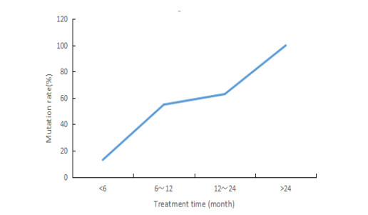
According to the mechanism of drug inhibition of hepatitis B virus and the analysis of clinical data, it is found that random factors in long-term treatment produced uncertainty and resistance to hepatitis B virus infection rate, a model of hepatitis B virus with random interference infection rate is established. By constructing Lyapunov function and using Ito's formula, it is proved that the stochastic hepatitis B model has a unique global positive solution. The sufficient conditions for the asymptotic behavior of solution are given. The relationship between noise intensity and oscillation amplitude is obtained. The effects of noise intensity on the asymptotic behavior of the model and antiviral therapy are simulated, and the conclusion of the theorem is verified. An interesting phenomenon is also found that with the increase of noise intensity, the number of drug-resistant viruses will decrease, which will affect the accuracy of a single test of HBV DNA. Therefore, it is suggested to increase the frequency and interval of tests.

References

[1]	J. Zhang, W. J. Xu, G. Wang, Analysis of lamivudine-resistant mutations in 268 patients with chronic hepatitis B during lamivudine therapy(In Chinese), Chin. J. Health Lab. Technol., 18 (2008), 2343–2344.
[2]	Y. Su, G. F. Gao, G. M. Li, Research progress on hepatitis B virus mutations and resistance to nucleosides, 2011. Available from: https://www.doc88.com/p-1963143564969.html.
[3]	J. Deng, X. X. Zhang, Nucleoside (acid) drug resistance mechanism and its countermeasures, Chin. J. Prac. Int. Med., 27 (2007), 1402–1404.
[4]	H. Y. Pang, W. D. Wang, Deterministic and stochastic analysis of a cell-to-cell virus dynamics model with immune impairment, J. Southwest Chin. Norm. Univ. (Nat. Sci. Ed.), 31 (2006), 26–30.
[5]	H. Y. Pang, W. D. Wang, Global properties of virus dynamics with CTL immune response, J. Southwest Chin. Norm. Univ. (Nat. Sci. Ed.), 30 (2005), 38–41.
[6]	F. L. Xie, M. J. Shan, X. Z. Lian, Periodic solution of a stochastic HBV infection model with logistic hepatocyte growth, Appl. Math. Comput., 293 (2017), 630–641.
[7]	Y. Wang, X. N. Liu, An HBV infection model with logistic growth, cure rate and CTL immune response, J. Southwest Chin. Norm. Univ. (Nat. Sci. Ed.), 38 (2016), 1–6.
[8]	H. W. Hui, The Analysis of Virus Model and Population Model with Stochastic Perturbation, MA. Thesis, Xinjiang University, 2018.
[9]	K. B. Bao, Q. M. Zhang, X. N. Li, A model of HBV infection with intervention strategies: dynamics analysis and numerical simulations, Math. Biosci. Eng., 16 (2019), 2562–2586. doi: 10.3934/mbe.2019129
[10]	Y. L. Cai, Y. Kang, M. Banerjee, W. M. Wang, A stochastic SIRS epidemic model with infectious force under intervention strategies, J. Differ. Equations, 259 (2015), 7463–7502. doi: 10.1016/j.jde.2015.08.024
[11]	Q. Liu, D. Q. Jiang, N. Z. Shi, T. Hayat, A. Alsaedi, Dynamical behavior of a stochastic HBV infection model with logistic hepatocyte growth, Acta Math. Sci., 37 (2017), 927–940. doi: 10.1016/S0252-9602(17)30048-6
[12]	M. Zhao, X. Y. Wang, Asymptotic behavior of global positive solution to stochastic SIQR epidemic model, J. Univ. Jinan (Sci. Technol.), 33 (2019), 88–94.
[13]	F. Y. Wei, Y. H. Cai. Y. H. Zhao, The asymptotic behavior of a stochastic SIQS epidemic model with nonlinear incidence, J. Biomath., 31 (2016), 109–117.
[14]	P. Y. Xia, The Dynamic Behavior of Several Stochastic Virus Models, Ph.D thesis, Northeast Normal University, 2018.
[15]	Y. N. Zhao, D. Q. Jiang, The extinction and persistence of the stochastic SIS epidemic model with vaccination, Phys. A Stat. Mech. Appl., 392 (2013), 4916–4927. doi: 10.1016/j.physa.2013.06.009
[16]	Y. Muroya, Y. Enatsu, H. Li, Global stability of a delayed HTLV–I infection model with a class of nonlinear incidence rates and CTLs immune response, Appl. Math. Comput., 219 (2013), 10559–10573.
[17]	X. W. Cui, Dynamic Behavior Analysis of Virus Infection Model Induced by Random Noise, MA. Thesis, Taiyuan University of Technology, 2018.
[18]	H. Srivastava, K. Saad, J. Gómez-Aguilar, A. A. Almadiy, Some new mathematical models of the fractional-order system of human immune against IAV infection, Math. Biosci. Eng., 17 (2020), 4942–4969. doi: 10.3934/mbe.2020268
[19]	K. Saad, J. Gómez–Aguilar, A. Almadiyd, A fractional numerical study on a chronic hepatitis C virus infection model with immune response, Chaos Solitons Fractals, 139 (2020), 110062. doi: 10.1016/j.chaos.2020.110062
[20]	H. Srivastava, K. Saad, Numerical simulation of the fractal-fractional Ebola virus, Fractal Fractional, 4 (2020), 49. doi: 10.3390/fractalfract4040049
[21]	D. M. Li, B. Chai, A dynamic model of hepatitis B virus with drug-resistant treatment, AIMS Math., 5 (2020), 4734–4753. doi: 10.3934/math.2020303
[22]	N. Wang, The research status of hepatitis B Virus cccDNA, Immunol. Studies, 3 (2015), 15–18.
[23]	X. Y. Liu, Q. H. Shang, X. S. Liu, Relationship between the serum HBV DNA and the change of the intrahepatic HBV cceDNA levels in antiviral therapy for chronic hepatitis B, Chin. Hepatol., 20 (2015), 591–596.
[24]	L. Min, Y. Su, Y. Kuang, Mathematical analysis of a basic virus infection model with application to HBV infection, Rocky Mt. J. Math., 38 (2008), 1573–1585.

Reader Comments

Your name:*

Email:*
© 2021 the Author(s), licensee AIMS Press. This is an open access article distributed under the terms of the Creative Commons Attribution License (http://creativecommons.org/licenses/by/4.0)