Getting to Zero (GTZ) initiatives focus on expanding use of antiretroviral treatment (ART) and pre-exposure prophylaxis (PrEP) to eliminate new HIV infections. Computational models help inform policies for implementation of ART and PrEP continuums. Such models, however, vary in their design, and may yield inconsistent predictions. Using multiple approaches can help assess the consistency in results obtained from varied modeling frameworks, and can inform optimal implementation strategies.
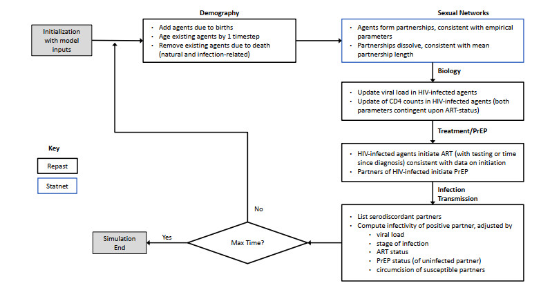
A study using three different modeling approaches is conducted. Two approaches use statistical time series analysis techniques that incorporate temporal HIV incidence data. A third approach uses stochastic stimulation, conducted using an agent-based network model (ABNM). All three approaches are used to project HIV incidence among a key population, young Black MSM (YBMSM), over the course of the GTZ implementation period (2016–2030).
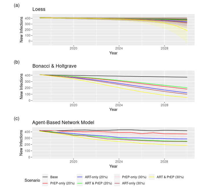
All three approaches suggest that simultaneously increasing PrEP and ART uptake is likely to be more effective than increasing only one, but increasing ART and PrEP by 20% points may not eliminate new HIV infections among YBMSM. The results further suggest that a 20% increase in ART is likely to be more effective than a 20% increase in PrEP. All three methods consistently project that increasing ART and PrEP by 30% simultaneously can help reach GTZ goals.
Increasing PrEP and ART uptake by about 30% might be necessary to accomplish GTZ goals. Such scale-up may require addressing psychosocial and structural barriers to engagement in HIV and PrEP care continuums. ABNMs and other flexible modeling approaches can be extended to examine specific interventions that address these barriers and may provide important data to guide the successful intervention implementation.
Citation: Aditya Subhash Khanna, Mert Edali, Jonathan Ozik, Nicholson Collier, Anna Hotton, Abigail Skwara, Babak Mahdavi Ardestani, Russell Brewer, Kayo Fujimoto, Nina Harawa, John A. Schneider. Projecting the number of new HIV infections to formulate the 'Getting to Zero' strategy in Illinois, USA[J]. Mathematical Biosciences and Engineering, 2021, 18(4): 3922-3938. doi: 10.3934/mbe.2021196
Getting to Zero (GTZ) initiatives focus on expanding use of antiretroviral treatment (ART) and pre-exposure prophylaxis (PrEP) to eliminate new HIV infections. Computational models help inform policies for implementation of ART and PrEP continuums. Such models, however, vary in their design, and may yield inconsistent predictions. Using multiple approaches can help assess the consistency in results obtained from varied modeling frameworks, and can inform optimal implementation strategies.
A study using three different modeling approaches is conducted. Two approaches use statistical time series analysis techniques that incorporate temporal HIV incidence data. A third approach uses stochastic stimulation, conducted using an agent-based network model (ABNM). All three approaches are used to project HIV incidence among a key population, young Black MSM (YBMSM), over the course of the GTZ implementation period (2016–2030).
All three approaches suggest that simultaneously increasing PrEP and ART uptake is likely to be more effective than increasing only one, but increasing ART and PrEP by 20% points may not eliminate new HIV infections among YBMSM. The results further suggest that a 20% increase in ART is likely to be more effective than a 20% increase in PrEP. All three methods consistently project that increasing ART and PrEP by 30% simultaneously can help reach GTZ goals.
Increasing PrEP and ART uptake by about 30% might be necessary to accomplish GTZ goals. Such scale-up may require addressing psychosocial and structural barriers to engagement in HIV and PrEP care continuums. ABNMs and other flexible modeling approaches can be extended to examine specific interventions that address these barriers and may provide important data to guide the successful intervention implementation.

| [1] | Joint United Nations Programme on HIV/AIDS (UNAIDS), Getting to Zero: 2011-2015 Strategy. 2010. Available from: http://files.unaids.org/en/media/unaids/contentassets/documents/unaidspublication/2010/20101221_JC2034E_UNAIDS-Strategy_en.pdf. |
| [2] | The White House, National HIV/AIDS strategy for the United States, Washington, DC, 2010. |
| [3] | National Alliance of State and Territorial AIDS Directors (NASTAD), Ending the HIV epidemic: jusrisdictional plans, Washington, D.C., 2018. Available from: https://www.nastad.org/maps/ending-hiv-epidemic-jurisdictional-plans. |
| [4] |
A. S. Fauci, H. D. Marston, Focusing to Achieve a World Without AIDS, JAMA, 313 (2015), 357-358. doi: 10.1001/jama.2014.17454

|
| [5] | J. R. Hargreaves, S. Delany-Moretlwe, T. B. Hallett, S. Johnson, S. Kapiga, P. Bhattacharjee, et al., The HIV prevention cascade: integrating theories of epidemiological, behavioural, and social science into programme design and monitoring, Lancet HIV, 7 (2016), e318-e322. |
| [6] |
A. Jones, I. Cremin, F. Abdullah, J. Idoko, P. Cherutich, N. Kilonzo, et al., Transformation of HIV from pandemic to low-endemic levels: a public health approach to combination prevention, Lancet, 384 (2014), 272-279. doi: 10.1016/S0140-6736(13)62230-8
|
| [7] |
B. C. Zanoni, K. H. Mayer, The adolescent and young adult HIV cascade of care in the United States: exaggerated health disparities, AIDS Patient Care STDS, 28 (2014), 128-135. doi: 10.1089/apc.2013.0345
|
| [8] | K. Risher, K. H. Mayer, C. Beyrer, HIV treatment cascade in MSM, people who inject drugs, and sex workers, Curr. Opin. HIV AIDS, 10 (2015), 420-429. |
| [9] | Centers for Disease Control and Prevention, HIV and Gay and Bisexual Men. Available from: https://www.cdc.gov/hiv/group/msm/index.html. |
| [10] | S. Cassels, S. J. Clark, M. Morris, Mathematical models for HIV transmission dynamics: tools for social and behavioral science research, J. Acquired Immune Defic. Syndr., 47 (2008), S34. |
| [11] |
E. T. Lofgren, M. E. Halloran, C. M. Rivers, J. M. Drake, T. C. Porco, B. Lewis, et al., Opinion: Mathematical models: A key tool for outbreak response, Proc. Natl. Acad. Sci., 111 (2014), 18095-18096. doi: 10.1073/pnas.1421551111
|
| [12] | S. M. Jenness, S. M. Goodreau, E. Rosenberg, E. N. Beylerian, K. W. Hoover, D. K. Smith, et al., Impact of the Centers for Disease Control's HIV Preexposure Prophylaxis Guidelines for Men Who Have Sex With Men in the United States, J. Infect. Dis., 214 (2016), 1800-1807. |
| [13] | S. M. Jenness, A. Sharma, S. M. Goodreau, E. S. Rosenberg, K. M. Weiss, K. W. Hoover, et al., Individual HIV risk versus population impact of risk compensation after HIV preexposure prophylaxis initiation among men who have sex with men, Plos One, 12 (2017), e0169484. |
| [14] |
W. C. Goedel, M. R. F. King, M. N. Lurie, A. S. Nunn, P. A. Chan, B. D. L. Marshall, Effect of Racial Inequities in Pre-Exposure Prophylaxis Use on Racial Disparities in HIV Incidence Among Men Who Have Sex with Men, J. Acquired Immune Defic. Syndr., 79 (2018), 323-329. doi: 10.1097/QAI.0000000000001817
|
| [15] | R. Brookmeyer, D. Boren, S. D. Baral, L. G. Bekker, N. Phaswana-Mafuya, C. Beyrer, et al., Combination HIV prevention among MSM in South Africa: results from agent-based modeling, Plos One, 9 (2014), e112668. |
| [16] | C. Celum, T. B. Hallett, J. M. Baeten, HIV-1 prevention with ART and PrEP: mathematical modeling insights into resistance, effectiveness, and public health impact, J. Infect. Dis., 208 (2013), 189-191. |
| [17] | A. A. King, M. Domenech de Cellès, F. M. G. Magpantay, P. Rohani, Avoidable errors in the modelling of outbreaks of emerging pathogens, with special reference to Ebola, Proc. R. Soc. B, 282 (2015), 20150347. |
| [18] |
A. S. Khanna, D. T. Dimitrov, S. M. Goodreau, What can mathematical models tell us about the relationship between circular migrations and HIV transmission dynamics?, Math. Biosci. Eng., 11 (2014), 1065-1090. doi: 10.3934/mbe.2014.11.1065
|
| [19] | V. A. Thurmond, The point of triangulation, J. Nurs. Scholarsh., 33 (2001), 253-258. |
| [20] | M. Leach, I. Scoones, The social and political lives of zoonotic disease models: Narratives, science and policy, Soc. Sci. Med., 88 (2013), 10-17. |
| [21] |
D. T. Campbell, D. W. Fiske, Convergent and discriminant validation by the multitrait-multimethod matrix, Psychol. Bull., 56 (1959), 81-105. doi: 10.1037/h0046016
|
| [22] |
J. C. Greene, V. J. Caracelli, W. F. Graham, Toward a conceptual framework for mixed-method evaluation designs, Educ. Eval. Policy Anal., 11 (1989), 255-274. doi: 10.3102/01623737011003255
|
| [23] | D. T. Halperin, O. Mugurungi, T. B. Hallett, B. Muchini, B. Campbell, T. Magure, et al., A Surprising Prevention Success: Why Did the HIV Epidemic Decline in Zimbabwe?, PLoS Med., 8 (2011), e1000414. |
| [24] |
G. W. Rutherford, W. McFarland, H. Spindler, K. White, S. V. Patel, J. Aberle-Grasse, et al., Public health triangulation: approach and application to synthesizing data to understand national and local HIV epidemics, BMC Public Health, 10 (2010), 447. doi: 10.1186/1471-2458-10-447
|
| [25] | J. W. Eaton, L. F. Johnson, J. A. Salomon, T. Barnighausen, E. Bendavid, A. Bershteyn, et al., HIV treatment as prevention: systematic comparison of mathematical models of the potential impact of antiretroviral therapy on HIV incidence in South Africa, Plos Med., 9 (2012), e1001245. |
| [26] |
D. A. M. C. van de Vijver, B. E. Nichols, U. L. Abbas, C. A. B. Boucher, V. Cambiano, J. W. Eaton, et al., Preexposure prophylaxis will have a limited impact on HIV-1 drug resistance in sub-Saharan Africa, AIDS, 27 (2013), 2943-2951. doi: 10.1097/01.aids.0000433237.63560.20
|
| [27] |
A. S. Khanna, J. A. Schneider, N. Collier, J. Ozik, R. Issema, A. di Paola, et al., A modeling framework to inform preexposure prophylaxis initiation and retention scale-up in the context of "Getting to Zero" initiatives, AIDS, 33 (2019), 1911-1922. doi: 10.1097/QAD.0000000000002290
|
| [28] | Getting to Zero Exploratory Workgroup, Getting To Zero: A Framework to Eliminate HIV in Illinois, 2017. Available from: https://www.aidschicago.org/resources/content/1/1/1/3/documents/GTZ_framework_August_draft.pdf. |
| [29] | Getting to Zero Exploratory Working Group. Getting to Zero: A Framework to Eliminate HIV in Illinois, Chicago, 2017. Available from: http://www.dph.illinois.gov/topics-services/diseases-and-conditions/hiv-aids/getting-zero. |
| [30] | Illinois Department of Public Health, Illinois Electronic HIV/ AIDS Reporting System. Available from: http://www.idph.state.il.us/ehrtf/ehrtf_home.htm. |
| [31] |
A. S. Khanna, S. Michaels, B. Skaathun, E. Morgan, K. Green, L. Young, et al., Preexposure prophylaxis awareness and use in a population-based sample of young black men who have sex with men, JAMA Intern. Med., 176 (2016), 136-138. doi: 10.1001/jamainternmed.2015.6536
|
| [32] | J. Schneider, B. Cornwell, A. Jonas, N. Lancki, R. Behler, B. Skaathun, et al., Network dynamics of HIV risk and prevention in a population-based cohort of young Black men who have sex with men, Network Sci., 2 (2017), 247. |
| [33] |
W. S. Cleveland, Robust locally weighted regression and smoothing scatterplots, J. Am. Stat. Assoc., 74 (1979), 829-836. doi: 10.1080/01621459.1979.10481038
|
| [34] | W. S. Cleveland, LOWESS: a program for smoothing scatterplots by robust locally weighted regression, Am. Stat., 35 (1981), 54. |
| [35] |
W. S. Cleveland, S. J. Devlin, Locally weighted regression: an approach to regression analysis by local fitting, J. Am. Stat. Assoc., 83 (1988), 596-610. doi: 10.1080/01621459.1988.10478639
|
| [36] |
J. R. Wong, J. K. Harris, C. Rodriguez-Galindo, K. J. Johnson, Incidence of childhood and adolescent melanoma in the United States: 1973-2009, Pediatrics, 131 (2013), 846-854. doi: 10.1542/peds.2012-2520
|
| [37] |
J. F. Ludvigsson, A. Rubio-Tapia, C. T. van Dyke, L. J. Melton, A. R. Zinsmeister, B. D. Lahr, et al., Increasing incidence of celiac disease in a north American population, Am. J. Gastroenterol., 108 (2013), 818-824. doi: 10.1038/ajg.2013.60
|
| [38] | J. M. Brotherton, M. Fridman, C. L. May, G. Chappell, A. M. Saville, D. M. Gertig, Early effect of the HPV vaccination programme on cervical abnormalities in Victoria, Australia: an ecological study, Lancet, 377 (2011), 2085-2092. |
| [39] | R. A. Bonacci, D. R. Holtgrave, Evaluating the impact of the US national HIV/AIDS strategy, 2010-2015, AIDS Behav., 20 (2016), 1383-1389. |
| [40] | S. C. Kalichman, Pence, Putin, Mbeki and their HIV/AIDS-related crimes against humanity: call for social justice and behavioral science advocacy, AIDS Behav., 27 (2017), 963-967. |
| [41] |
D. R. Holtgrave, R. A. Bonacci, R. O. Valdiserri, Presidential elections and HIV-related national policies and programs, AIDS Behav., 21 (2017), 611-614. doi: 10.1007/s10461-017-1703-z
|
| [42] | H. I. Hall, R. Song, T. Tang, Q. An, J. Prejean, P. Dietz, et al., HIV trends in the United States: Diagnoses and Estimated Incidence, JMIR Public Heal Surveill., 3 (2017), e8. |
| [43] | R. O. Valdiserri, C. H. Maulsby, D. R. Holtgrave, Structural factors and the national HIV/AIDS strategy of the USA, Struct. Dyn. HIV, (2018), 173-194. |
| [44] |
G. Robins, T. Snijders, P. Wang, M. Handcock, P. Pattison, Recent developments in exponential random graph (p*) models for social networks, Soc. Networks., 29 (2007), 192-215. doi: 10.1016/j.socnet.2006.08.003
|
| [45] | Statnet Development Team (Pavel N. Krivitsky, Mark S. Handcock, David R. Hunter, Carter T. Butts, Chad Klumb, Steven M. Goodreau, and Martina Morris) (2003-2020). statnet: Software tools for the Statistical Modeling of Network Data. URL http://statnet.org |
| [46] |
N. Collier, M. North, Parallel agent-based simulation with repast for High Performance Computing, Simulation, 89 (2013), 1215-1235. doi: 10.1177/0037549712462620
|
| [47] | N. Collier, J. T. Murphy, J. Ozik, E. Tatara, Repast for High Performance Computing, 2018. Available from: https://repast.github.io/repast_hpc.html. |
| [48] | A. S. Khanna, N. Collier, J. Ozik, BARS: Building Agent-based Models for Racialized Justice Systems, 2017. Available from: https://github.com/khanna7/BARS. |
| [49] | D. R. Holtgrave, H. I. Hall, L. Wehrmeyer, C. Maulsby, Costs, Consequences and Feasibility of Strategies for Achieving the Goals of the National HIV/AIDS Strategy in the United States: A Closing Window for Success?, AIDS Behav., 16 (2012), 1365-1372. |
| [50] |
J. Koopman, Modeling infection transmission, Annu. Rev. Public Health, 25 (2004), 303-326. doi: 10.1146/annurev.publhealth.25.102802.124353
|
| [51] |
J. S. Koopman, Modeling infection transmission-the pursuit of complexities that matter, Epidemiology, 13 (2002), 622-624. doi: 10.1097/00001648-200211000-00004
|
| [52] | R. A. Bonacci, D. R. Holtgrave, U.S. HIV incidence and transmission goals, 2020 and 2025, Am. J. Prev. Med., 53 (2017), 275-281. |
| [53] |
T. M. Hammett, J. L. Gaiter, C. Crawford, Reaching seriously at-risk populations: health interventions in criminal justice settings, Health Educ. Behav., 25 (1998), 99-120. doi: 10.1177/109019819802500108
|
| [54] | L. Bowleg, M. Teti, D. J. Malebranche, J. M. Tschann, "It's an Uphill Battle Everyday": intersectionality, low-income black heterosexual men, and implications for HIV prevention research and interventions, Psychol. Men Masculinity, 14 (2013), 25-34. |
| [55] |
R. A. Jenkins, Getting to zero: we can't do it without addressing substance use, AIDS Educ. Prev., 30 (2018), 225-231. doi: 10.1521/aeap.2018.30.3.225
|
| [56] | J. Seeley, C. H. Watts, S. Kippax, S. Russell, L. Heise, A. Whiteside, Addressing the structural drivers of HIV: a luxury or necessity for programmes?, J. Int. AIDS Soc., 15 (2012). |
| [57] | D. V. Havlir, S. P. Buchbinder, Ending AIDS in the United States-if not now, when?, JAMA Intern. Med., 179 (2019), 1165-1166. |
| [58] | E. H. Layer, C. E. Kennedy, S. W. Beckham, J. K. Mbwambo, S. Likindikoki, W. W. Davis, et al., Multi-level factors affecting entry into and engagement in the HIV continuum of care in Iringa, Tanzania, Plos One, 9 (2014), e104961. |
| [59] | C. H. Logie, V. L. Kennedy, W. Tharao, U. Ahmed, M. R. Loutfy, Engagement in and continuity of HIV care among African and Caribbean black women living with HIV in Ontario, Canada, Int. J. STD AIDS, 28 (2017), 969-974. |
| [60] | O. Bonnington, J. Wamoyi, W. Ddaaki, D. Bukenya, K. Ondenge, M. Skovdal, et al., Changing forms of HIV-related stigma along the HIV care and treatment continuum in sub-Saharan Africa: a temporal analysis, Sex. Trans. Infect., 93 (2017), e052975. |
| [61] | R. Sutton, M. Lahuerta, F. Abacassamo, L. Ahoua, M. Tomo, M. R. Lamb, et al., Feasibility and acceptability of health communication interventions within a combination intervention strategy for improving linkage and retention in HIV care in Mozambique, J. Acquired Immune Defic. Syndr., 74 (2017), S29-S36. |
| [62] | C. H. Brown, D. C. Mohr, C. G. Gallo, C. Mader, L. Palinkas, G. Wingood, et al., A computational future for preventing HIV in minority communities: how advanced technology can improve implementation of effective programs, J. Acquired Immune Defic. Syndr., 63 (2013), S72-S84. |
| [63] | R Core Team, The R project for statistical computing, 2019. Available from: https://www.r-project.org/. |
| [64] |
A. Y. Liu, S. E. Cohen, E. Vittinghoff, P. L. Anderson, S. Doblecki-Lewis, O. Bacon, et al., Preexposure prophylaxis for HIV infection integrated with municipal- and community-based sexual health services, JAMA Intern. Med., 176 (2016), 75-84. doi: 10.1001/jamainternmed.2015.4683
|
| [65] |
L. K. Rusie, C. Orengo, D. Burrell, A. Ramachandran, M. Houlberg, K. Keglovitz, et al., Preexposure prophylaxis initiation and retention in care over 5 years, 2012-2017: are quarterly visits too much?, Clin. Infect. Dis., 67 (2018), 283-287. doi: 10.1093/cid/ciy160
|

Figures(3) / Tables(1)

Aditya Subhash Khanna, Mert Edali, Jonathan Ozik, Nicholson Collier, Anna Hotton, Abigail Skwara, Babak Mahdavi Ardestani, Russell Brewer, Kayo Fujimoto, Nina Harawa, John A. Schneider. Projecting the number of new HIV infections to formulate the "Getting to Zero" strategy in Illinois, USA[J]. Mathematical Biosciences and Engineering, 2021, 18(4): 3922-3938. doi: 10.3934/mbe.2021196


 DownLoad: