Design and analysis of a robust breast cancer diagnostic system based on multimode MR images

Hong Yu; Wenhuan Lu; Qilong Sun; Haiqiang Shi; Jianguo Wei; Zhe Wang; Xiaoman Wang; Naixue Xiong; Hong Yu; Wenhuan Lu; Qilong Sun; Haiqiang Shi; Jianguo Wei; Zhe Wang; Xiaoman Wang; Naixue Xiong

doi:10.3934/mbe.2021180

Mathematical Biosciences and Engineering

2021, Volume 18, Issue 4: 3578-3597. doi: 10.3934/mbe.2021180

Previous Article Next Article

Research article Special Issues

Design and analysis of a robust breast cancer diagnostic system based on multimode MR images

1.
Center Obstetrics and Gynecology Hospital, Tianjin 300100, China
2.
College of Intelligence and Computing, Tianjin University, Tianjin 300350, China
3.
School of Computer Science, Qinghai Nationalities University, Xining Qinghai, 810007, China
4.
Qinghai Provincial Party School, Xining Qinghai, 810007, China
5.
IBM China Company Limited, Beijing 100193, China

Received: 21 October 2020 Accepted: 22 February 2021 Published: 25 April 2021

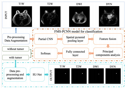
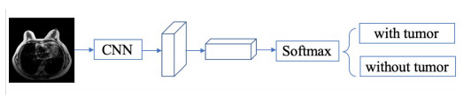
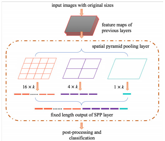
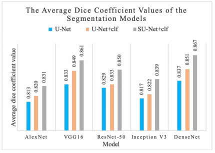
In this paper, we propose a Robust Breast Cancer Diagnostic System (RBCDS) based on multimode Magnetic Resonance (MR) images. Firstly, we design a four-mode convolutional neural network (FMS-PCNN) model to detect whether an image contains a tumor. The features of the images generated by different imaging modes are extracted and fused to form the basis of classification. This classification model utilizes both spatial pyramid pooling (SPP) and principal components analysis (PCA). SPP enables the network to process images of different sizes and avoids the loss due to image resizing. PCA can remove redundant information in the fused features of multi-sequence images. The best accuracy of this model achieves 94.6%. After that, we use our optimized U-Net (SU-Net) to segment the tumor from the entire image. The SU-Net achieves a mean dice coefficient (DC) value of 0.867. Finally, the performance of the system is analyzed to prove that this system is superior to the existing schemes.
- classification,
- convolutional neural networks,
- Magnetic Resonance imaging,
- multiple modes,
- segmentation
Citation: Hong Yu, Wenhuan Lu, Qilong Sun, Haiqiang Shi, Jianguo Wei, Zhe Wang, Xiaoman Wang, Naixue Xiong. Design and analysis of a robust breast cancer diagnostic system based on multimode MR images[J]. Mathematical Biosciences and Engineering, 2021, 18(4): 3578-3597. doi: 10.3934/mbe.2021180

Related Papers:

Abstract

In this paper, we propose a Robust Breast Cancer Diagnostic System (RBCDS) based on multimode Magnetic Resonance (MR) images. Firstly, we design a four-mode convolutional neural network (FMS-PCNN) model to detect whether an image contains a tumor. The features of the images generated by different imaging modes are extracted and fused to form the basis of classification. This classification model utilizes both spatial pyramid pooling (SPP) and principal components analysis (PCA). SPP enables the network to process images of different sizes and avoids the loss due to image resizing. PCA can remove redundant information in the fused features of multi-sequence images. The best accuracy of this model achieves 94.6%. After that, we use our optimized U-Net (SU-Net) to segment the tumor from the entire image. The SU-Net achieves a mean dice coefficient (DC) value of 0.867. Finally, the performance of the system is analyzed to prove that this system is superior to the existing schemes.

References

[1]	R. L. Siegel, K. D. Miller, A. Jemal, Cancer Statistics, 2019, Cancer J. Clin., 69 (2019), 7–34.
[2]	K. Deike‐Hofmann, F. Koenig, D. Paech, C. Dreher, S. Delorme, H. Schlemmer, et al., Abbreviated MRI Protocols in Breast Cancer Diagnostics, J Magn. Reson. Imaging, 49 (2019), 647–658. doi: 10.1002/jmri.26525
[3]	H. Chougrad, H. Zouaki, O. Alheyane, Deep Convolutional Neural Networks for breast cancer screening, Comput. Mehtod Prog. Biomed., 157 (2018), 19–30. doi: 10.1016/j.cmpb.2018.01.011
[4]	A Gubernmrida, M Kallenberg, R. M. Mann, R Mart, N Karssemeijer, Breast segmentation and density estimation in breast MRI: a fully automatic framework, IEEE J. Biomed. Health Infor., 19 (2015), 349–357. doi: 10.1109/JBHI.2014.2311163
[5]	R. M. Mann, N. Cho, L. Moy, Breast MRI: State of the Art, Radiology, 292 (2019), 520–536. doi: 10.1148/radiol.2019182947
[6]	C. D. Lehman, R. D. Wellman, D. S. M. Buist, Diagnostic Accuracy of Digital Screening Mammography With and Without Computer-Aided Detection, JAMA Int. Med., 175 (2015), 1828–1837. doi: 10.1001/jamainternmed.2015.5231
[7]	T. Kyono, F. J. Gilbert, M. van der Schaar, MAMMO: A Deep Learning Solution for Facilitating Radiologist-Machine Collaboration in Breast Cancer Diagnosis, preprint, arXiv: 1811.02661.
[8]	F. A. Maken, A. P. Bradley, Multiple Instance Learning for Breast MRI Based on Generic Spatio-temporal Features, 2015 IEEE International Conference on Acoustics, Speech and Signal Processing (ICASSP), 2015.
[9]	Y. Lecun, Y. Bengio, G. Hinton, Deep learning, Nature, 521 (2015), 436–444.
[10]	C. Szegedy, W. Liu, Y. Jia, P. Sermanet, S. Reed, D. Anguelov, et al., Going Deeper with Convolutions, Proceedings of the IEEE Conference on Computer Vision and Pattern Recognition (CVPR), 2015.
[11]	Z. Fang, F. Fei, Y. Fang, C. Lee, N. Xiong, L. Shu, et al., Abnormal event detection in crowded scenes based on deep learning, Multimed Tools Appl., 75 (2016), 14617–14639. doi: 10.1007/s11042-016-3316-3
[12]	A. Krizhevsky, I. Sutskever, G. E. Hinton, ImageNet classification with deep convolutional neural networks, Adv. Neural Inf. Process. Syst., 25 (2012), 1097–1105.
[13]	J. Long, E. Shelhamer, T. Darrell, Fully Convolutional Networks for Semantic Segmentation, Proceedings of the IEEE Conference on Computer Vision and Pattern Recognition (CVPR), 2015.
[14]	Q. Hu, C. Wu, Y. Wu, N. Xiong, UAV Image High Fidelity Compression Algorithm Based on Generative Adversarial Networks Under Complex Disaster Conditions, IEEE Access, 7 (2019), 91980–91991. doi: 10.1109/ACCESS.2019.2927809
[15]	Y. Xu, H. Yang, J. Li, J. Liu, N. Xiong, An Effective Dictionary Learning Algorithm Based on fMRI Data for Mobile Medical Disease Analysis, IEEE Access, 7 (2018), 3958–3966.
[16]	C. Wu, C. Luo, N. Xiong, W. Zhang, T. H. Kim, A Greedy Deep Learning Method for Medical Disease Analysis, IEEE Access, 6 (2018), 20021–20030. doi: 10.1109/ACCESS.2018.2823979
[17]	D. Truhn, S. Schrading, C. Haarburger, H. Schneider, D. Merhof, C. Kuhl, Radiomic versus Convolutional Neural Networks Analysis for Classification of Contrast-enhancing Lesions at Multiparametric Breast MRI, Radiology, 290 (2019), 290–297. doi: 10.1148/radiol.2018181352
[18]	N. Chen, T. Qiu, X. Zhou, K. Li, M. Atiquzzaman, An Intelligent Robust Networking Mechanism for the Internet of Things, IEEE Commun. Mag., 57 (2019), 91–95.
[19]	T. Qiu, J. Liu, W. Si, D. O. Wu, Robustness optimization scheme with multi-population co-evolution for scale-free wireless sensor networks, IEEE Trans. Networking, 27 (2019), 1028–1042. doi: 10.1109/TNET.2019.2907243
[20]	T. Qiu, B. Li, W. Qu, E. Ahmed, X. Wang, TOSG: A topology optimization scheme with global-small-world for industrial heterogeneous Internet of Things, IEEE Trans. Ind. Inf., 15 (2019), 3174–3184. doi: 10.1109/TII.2018.2872579
[21]	K. He, X. Zhang, S. Ren, J. Sun, Spatial Pyramid Pooling in Deep Convolutional Networks for Visual Recognition, IEEE Trans. Pattern Anal. Mach. Intell., 37 (2015), 1904–1916. doi: 10.1109/TPAMI.2015.2389824
[22]	N. N Mohammed, M. I. Khaleel, M. Latif, Z. Khalid, Face Recognition Based on PCA with Weighted and Normalized Mahalanobis distance, 2018 International Conference on Intelligent Informatics and Biomedical Sciences (ICIIBMS), 2018.
[23]	W. Lu, Z. Wang, Y. He, H. Yu, N. Xiong, J. Wei, Breast Cancer Detection Based On Merging Four Modes MRI Using Convolutional Neural Networks, ICASSP 2019-2019 IEEE International Conference on Acoustics, Speech and Signal Processing (ICASSP), 2019.
[24]	O. Ronneberger, P. Fischer, T. Brox, U-Net: Convolutional Networks for Biomedical Image Segmentation, International Conference on Medical Image Computing and Computer-Assisted Intervention, 2015.
[25]	W. Shi, J. Caballero, F. Huszar, J. Totz, A. P. Aitken, R. Bishop, et al., Real-Time Single Image and Video Super-Resolution Using an Efficient Sub-Pixel Convolutional Neural Network, Proceedings of the IEEE Conference on Computer Vision and Pattern Recognition (CVPR), 2016.
[26]	F. A. Spanhol, L. S. Oliveira, C. Petitjean, L. Heutte, Breast Cancer Histopathological Image Classification using Convolutional Neural Networks, 2016 International Joint Conference on Neural Networks (IJCNN), 2016.
[27]	Y. Wen, K. Zhang, Z. Li, Y. Qiao, A Discriminative Feature Learning Approach for Deep Face Recognition, European Conference on Computer Vision, 2016.
[28]	Y. Gao, X. Xiang, N. Xiong, B. Huang, H. Jong Lee, R. Alrifai, et al., Human Action Monitoring for Healthcare Based on Deep Learning, IEEE Access, 6 (2018), 52277–52285. doi: 10.1109/ACCESS.2018.2869790
[29]	K. He, X. Zhang, S. Ren, J. Sun, Deep Residual Learning for Image Recognition, Proceedings of the IEEE Conference on Computer Vision and Pattern Recognition (CVPR), 2016.
[30]	Z. Wang, W. Lu, Y. He, N. Xiong, J. Wei, RE-CNN: A Robust Convolutional Neural Networks for Image Recognition, International Conference on Neural Information Processing, 2018.
[31]	K. Simonyan, A. Zisserman, Very Deep Convolutional Networks for Large-Scale Image Recognition, preprint, arXiv: 1409.1556.
[32]	B. Zhou, A. Khosla, A. Lapedriza, A. Oliva, A. Torralba, Object Detectors Emerge in Deep Scene CNNs, preprint, arXiv: 1412.6856.
[33]	B. Zhou, A. Lapedriza, J. Xiao, A. Torralba, A. Oliva, Learning Deep Features for Scene Recognition Using Places Database, Proceedings of the 27th International Conference on Neural Information Processing Systems, 2014.
[34]	S. Liu, J. Zeng, H. Gong, H. Yang, J. Zhai, Y. Cao, et al., Quantitative analysis of breast cancer diagnosis using a probabilistic modelling approach, Comput. Biol. Med., 92 (2018), 168–175. doi: 10.1016/j.compbiomed.2017.11.014
[35]	A. M. Sayed, E. Zaghloul, T. M. Nassef, Automatic classification of breast tumors using features extracted from magnetic resonance images, Procedia Comput. Sci., 95 (2016), 392–398. doi: 10.1016/j.procs.2016.09.350
[36]	K. Drukker, R. Anderson, A. Edwards, J. Papaioannou, F. Pineda, H. Abe, et al., Radiomics for Ultrafast Dynamic Contrast-Enhanced Breast MRI in the Diagnosis of Breast Cancer: a Pilot Study, Medical Imaging 2018: Computer-Aided Diagnosis. International Society for Optics and Photonics, 2018,
[37]	G. Maicas, G. Carneiro, A. P. Bradley, Globally Optimal Breast Mass Segmentation from DCE-MRI Using Deep Semantic Segmentation as Shape Prior, 2017 IEEE 14th International Symposium on Biomedical Imaging, 2017.
[38]	J. Zhang, A. Saha, Z. Zhu, M. A. Mazurowski, Breast Tumor Segmentation in DCE-MRI Using Fully Convolutional Networks with an Application in Radiogenomics, Medical Imaging 2018: Computer-Aided Diagnosis. International Society for Optics and Photonics, 2018.
[39]	M. Z. Alom, M. Hasan, C. Yakopcic, T. M. Taha, V. K. Asari, Recurrent Residual Convolutional Neural Network based on U-Net (R2U-Net) for Medical Image Segmentation, preprint, arXiv: 1802.06955.
[40]	Z. Zhou, M. M. R. Siddiquee, N. Tajbakhsh, J. Liang, UNet++: A Nested U-Net Architecture for Medical Image Segmentation, Deep Learning in Medical Image Analysis and Multimodal Learning for Clinical Decision Support, 2018.
[41]	F. Isensee, P. Kickingereder, W. Wick, M. Bendszus, K. H. M. Hein. No New-net, Brainlesion: Glioma, Multiple Sclerosis, Stroke and Traumatic Brain Injuries, 2018.
[42]	H. C. Shin, H. R. Roth, M. Gao, L. Lu, Z. Xu, I Nogues, et al., Deep Convolutional Neural Networks for Computer-Aided Detection: CNN Architectures, Dataset Characteristics and Transfer Learning, IEEE Trans. Med. Imaging, 35 (2016), 1285–1298. doi: 10.1109/TMI.2016.2528162
[43]	N. Amornsiripanitch, S. Bickelhaupt, H. J. Shin, M. Dang, H. Rahbar, K. Pinker, et al., Diffusion-weighted MRI for Unenhanced Breast Cancer Screening, Radiology, 293 (2019), 504–520. doi: 10.1148/radiol.2019182789
[44]	H. Hu, J. Gu, Z. Zhang, J. Dai, Y. Wei, Relation Networks for Object Detection, Proceedings of the IEEE Conference on Computer Vision and Pattern Recognition (CVPR), 2018.
[45]	X. Lu, X. Duan, X. Mao, Y. Li, X. Zhang, Feature Extraction and Fusion Using Deep Convolutional Neural Networks for Face Detection, Math. Prob. Eng., 2017 (2017), 1376726.
[46]	C. Szegedy, V. Vanhoucke, S. Ioffe, J. Shlens, Z. Wojna, Rethinking the Inception Architecture for Computer Vision, Proceedings of the IEEE Conference on Computer Vision and Pattern Recognition (CVPR), 2016.
[47]	G. Huang, Z. Liu, L. van der Maaten, K. Q. Weinberger, Densely Connected Convolutional Networks, Proceedings of the IEEE Conference on Computer Vision and Pattern Recognition (CVPR), 2017.
[48]	W. Shi, J. Caballero, C. Ledig, X. Zhuang, W. Bai, K. Bhatia, et al., Cardiac Image Super-Resolution with Global Correspondence Using Multi-Atlas PatchMatch, Medical Image Computing and Computer-Assisted Intervention, MICCAI 2013.
[49]	C. Haarburger, M. Baumgartner, D. Truhn, M. Broeckmann, H. Schneider, S. Schrading, et al., Multi Scale Curriculum CNN for Context-Aware Breast MRI Malignancy Classification, Medical Image Computing and Computer Assisted Intervention, MICCAI 2019.
[50]	F. F. Ting, Y. J. Tan, K. S. Sim, Convolutional neural network improvement for breast cancer classification, Expert Syst. Appl., 120 (2019), 103–115. doi: 10.1016/j.eswa.2018.11.008
[51]	G. Maicas, A. P. Bradley, J. C. Nascimento, I. Reid, G. Carneiro, Training Medical Image Analysis Systems like Radiologists, Medical Image Computing and Computer Assisted Intervention, MICCAI 2018.
[52]	S. Marrone, G. Piantadosi, R. Fusco, A. Petrillo, M. Sansone, C. Sansone, Breast Segmentation Using Fuzzy C-Means and Anatomical Priors in DCE-MRI, 2016 23rd International Conference on Pattern Recognition (ICPR), 2016.
[53]	J. Long, E. Shelhamer, T. Darrell, Fully Convolutional Networks for Semantic Segmentation, Proceedings of the IEEE Conference on Computer Vision and Pattern Recognition (CVPR), 2015.
[54]	V. Badrinarayanan, A. Kendall, R. Cipolla, SegNet: A Deep Convolutional Encoder-Decoder Architecture for Image Segmentation, IEEE Trans Pattern Anal. Mach. Intell., 39 (2017), 2481–2495. doi: 10.1109/TPAMI.2016.2644615

Reader Comments

Your name:*

Email:*
© 2021 the Author(s), licensee AIMS Press. This is an open access article distributed under the terms of the Creative Commons Attribution License (http://creativecommons.org/licenses/by/4.0)