A mathematical model for Vibrio-phage interactions

Christopher Botelho; Jude Dzevela Kong; Mentor Ali Ber Lucien; Zhisheng Shuai; Hao Wang; Christopher Botelho; Jude Dzevela Kong; Mentor Ali Ber Lucien; Zhisheng Shuai; Hao Wang

doi:10.3934/mbe.2021137

Mathematical Biosciences and Engineering

2021, Volume 18, Issue 3: 2688-2712. doi: 10.3934/mbe.2021137

Previous Article Next Article

Research article

A mathematical model for Vibrio-phage interactions

1.
Department of Mathematics, University of Central Florida, Orlando, Florida, 32816, USA
2.
Department of Mathematics and Statistics, York University, Toronto, Ontario, M3J 1P3, Canada
3.
The Canadian Center for Disease Modelling, York University, Toronto, Ontario, M3J 1P3, Canada
4.
Laboratoire National de Santé Publique, Ministère de la Santé Publique et de la Population d'Haiti, Port-au-Prince, HT6120, Haiti
5.
Department of Mathematical and Statistical Sciences, University of Alberta, Edmonton, Alberta, T6G 2G1, Canada

Received: 29 October 2020 Accepted: 18 February 2021 Published: 19 March 2021

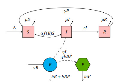
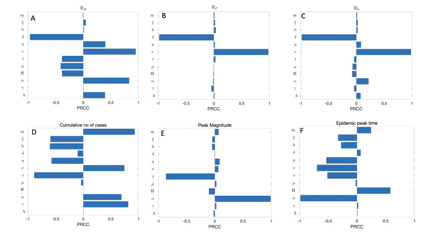
A cholera model has been formulated to incorporate the interaction of bacteria and phage. It is shown that there may exist three equilibria: one disease free and two endemic equilibria. Threshold parameters have been derived to characterize stability of these equilibria. Sensitivity analysis and disease control strategies have been employed to characterize the impact of bacteria-phage interaction on cholera dynamics.
- cholera,
- bacteriophage,
- global stability,
- basic reproduction number
Citation: Christopher Botelho, Jude Dzevela Kong, Mentor Ali Ber Lucien, Zhisheng Shuai, Hao Wang. A mathematical model for Vibrio-phage interactions[J]. Mathematical Biosciences and Engineering, 2021, 18(3): 2688-2712. doi: 10.3934/mbe.2021137

Related Papers:

Abstract

A cholera model has been formulated to incorporate the interaction of bacteria and phage. It is shown that there may exist three equilibria: one disease free and two endemic equilibria. Threshold parameters have been derived to characterize stability of these equilibria. Sensitivity analysis and disease control strategies have been employed to characterize the impact of bacteria-phage interaction on cholera dynamics.

References

[1]	R. A. Finkelstein, Cholera, Vibrio cholerae O1 and O139 and other pathogenic vibrios. In: S. Baron (Ed.), Medical Microbiology, 4th edition, University of Texas, Galveston, TX, 1996, Ch. 24.
[2]	WHO (2019). Cholera, fact sheet. available from: https://www.who.int/en/news-room/fact-sheets/detail/cholera retrieved on July 12, 2019.
[3]	M. A. B. Lucien, P. Adrien, H. Hadid, T. Hsia, M. F. Canarie, L. M. Kaljee, et al., Cholera outreak in Haiti: Epidemiology, Control, and Prevention, Infect. Dis. Clin. Practice, 27 (2019), 3–11. doi: 10.1097/IPC.0000000000000684
[4]	WHO. Weekly epidemiological record. Number 38 (2016) 433–440.
[5]	T. Ramamurthy, A. Ghosh, G. P. Pazhani, S. Shinoda, Current perspectives on viable but non-culturable (VBNC) pathogenic bacteria, Front. Public Health, 2 (2014), 103.
[6]	C. T. Codeço, Endemic and epidemic dynamics of cholera: The role of the aquatic reservoir, BMC Infect. Dis., 1 (2001), 1–14. doi: 10.1186/1471-2334-1-1
[7]	K. Kierek, P. I. Watnick, Environmental determinants of Vibrio cholerae biofilm development, Appl. Environ. Microbiol., 69 (2003), 5079–5088. doi: 10.1128/AEM.69.9.5079-5088.2003
[8]	M. A. Jensen, S. M. Faruque, J. J. Mekalanos, B. R. Levin, Modeling the role of bacteriophage in the control of cholera outbreaks, P. Natl. Acad. Sci. USA, 103 (2006), 4652–4657. doi: 10.1073/pnas.0600166103
[9]	J. D. Kong, W. Davis, H. Wang, Dynamics of a cholera transmission model with immunological threshold and natural phage control in reservoir, Bull. Math. Biol., 76 (2014), 2025–2051. doi: 10.1007/s11538-014-9996-9
[10]	A. A. King, E. L. Ionides, M. Pascual, M. J. Buoma, Inapparent infections and cholera dynamics, Nature, 454 (2008), 877–890. doi: 10.1038/nature07084
[11]	M. Levine, R. Black, M. Clements, L. Cisneros, D. Nalin, C. Young, Duration of infection-derived immunity to cholera, J. Infect. Dis., 143 (1981), 818–820. doi: 10.1093/infdis/143.6.818
[12]	R. P. Sanches, C. P. Ferreira, R. Kraenkel, The Role of immunity and seasonality in cholera epidemics, Bull. Math. Biol., 73 (2011), 2916–2931. doi: 10.1007/s11538-011-9652-6
[13]	J. H. Tien, D. J. D. Earn, Multiple transmission pathways and disease dynamics in a waterborne pathogen model, Bull. Math. Biol., 72 (2010), 1506–1533. doi: 10.1007/s11538-010-9507-6
[14]	M. Bani-Yaghoub, R. Gautam, Z. Shuai, P. van den Driessche, R. Ivanek, Reproduction numbers for infections with free-living pathogens growing in the environment, J. Biol. Dyn., 6 (2012), 923–940. doi: 10.1080/17513758.2012.693206
[15]	J. P. LaSalle, The Stability of Dynamical Systems, Regional Conference Series in Applied Mathematics, SIAM, Philadelphia, PA, 1976.
[16]	O. Diekmann, J. A. Heesterbeek, M. G. Roberts, The construction of next-generation matrices for compartmental epidemic models, J. R. Soc. Interface, 7 (2010), 873–885. doi: 10.1098/rsif.2009.0386
[17]	P. van den Driessche, J. Watmough, Reproduction numbers and sub-threshold endemic equilibria for compartmental models of disease transmission, Math. Biosci., 180 (2002), 29–48. doi: 10.1016/S0025-5564(02)00108-6
[18]	M. A. Lewis, Z. Shuai, P. van den Driessche, A general theory for target reproduction numbers with applications to ecology and epidemiology, J. Math. Biol., 78 (2019), 2317–2339. doi: 10.1007/s00285-019-01345-4
[19]	A. Lupica, A. B. Gumel, A. Palumbo, Computation of reproduction numbers for the environment-host-environment cholera transmission dynamics, J. Biol. Syst., 28 (2020), 1–49.
[20]	M. D. McKay, R. J. Beckman, W. J. Conover, A comparison of three methods for selecting values of input variables in the analysis of output from a computer code, Technometrics, 21 (1979), 239–245.
[21]	Z. Shuai, J. A. P. Heesterbeek, P. van den Driessche, Extending the type reproduction number to infectious disease control targeting contacts between types, J. Math. Biol., 67 (2013), 1067–1082. Also the erratum, J. Math. Biol., 71 (2015), 255–257.
[22]	C. Yang, J. Wang, On the intrinsic dynamics of bacteria in waterborne infections, Math. Biosci., 296 (2018), 71–81. doi: 10.1016/j.mbs.2017.12.005
[23]	I. C.-H. Fung, Cholera transmission dynamic models for public health practitioners, Emerg. Themes Epidemiology, 11 (2014), 1–14. doi: 10.1186/1742-7622-11-1
[24]	M. Phelps, M. L. Perner, V. E. Pitzer, V. Andreasen, P. K. M. Jensen, L. Simonsen, Cholera epidemics of the past offer new insights into an old enemy, J. Infect. Diseases, 217 (2018), 641–649. doi: 10.1093/infdis/jix602
[25]	D. M. Hartley, J. G. Morris Jr., D. L. Smith, Hyperinfectivity: a critical element in the ability of V. cholerae to cause epidemics?, PLOS Med., 3 (2006), 63. doi: 10.1371/journal.pmed.0030063
[26]	M. Eisenberg, S. L. Robertson, J. H. Tien, Identifiability and estimation of multiple transmission pathways in cholera and waterborne disease, J. Theor. Biol., 324 (2013), 84–102. doi: 10.1016/j.jtbi.2012.12.021
[27]	S. M. Blower, H. Dowlatabadi, Sensitivity and uncertainty analysis of Complex models of disease transmission: an HIV Model, as an example, Int. Stat. Rev., 62 (1994), 229–243. doi: 10.2307/1403510
[28]	P. A. Blake, Historical perspectives on pandemic cholera, Vibrio cholerae and cholera, American Society for Microbiology, Washington, DC, 1994,293–295.
[29]	R. M. Donlan, Biofilms: Microbial Life on Surfaces, Emerging Infect. Dis., 8 (2002), 881–890. doi: 10.3201/eid0809.020063
[30]	L. Li, N. Mendis, H. Trigui, J. D. Oliver, S. P. Faucher, The importance of the viable but non-culturable state in human bacterial pathogens, Front. Microbiol., 5 (2014), 258.
[31]	J. D. Murray, Mathematical Biology I: An Introduction. 3rd edition. Springer, NY, 2002.
[32]	A. K. Misra, A. Gupta, E. Venturino, Cholera dynamics with bacteriophage infection: a mathematical study, Chaos Solitons Fract., 91 (2016), 610–621. doi: 10.1016/j.chaos.2016.08.008
[33]	A. J. Silva, J. A. Benitez, Vibrio cholerae biofilms and cholera pathogenesis, PLoS Negl. Trop. Dis., 10 (2016), e0004330. doi: 10.1371/journal.pntd.0004330
[34]	A. Solís-Sánchez, U. Hernández-Chiñas, A. Navarro-Ocaña, L. M. De, J. Xicohtencatl-Cortes, C. Eslava-Campos, Genetic characterization of ØVC8 lytic phage for Vibrio cholerae O1, Virol. J., 13 (2016), 47.
[35]	J. K. Teschler, D. Zamorano-Sánchez, A. S. Utada, C. J. Warner, G. C. Wong, R. G. Linington, et al., Living in the matrix: assembly and control of Vibrio cholerae biofilms, Nat. Rev. Microbiol., 13 (2015), 255–268. doi: 10.1038/nrmicro3433

Reader Comments

Your name:*

Email:*
© 2021 the Author(s), licensee AIMS Press. This is an open access article distributed under the terms of the Creative Commons Attribution License (http://creativecommons.org/licenses/by/4.0)