Processing math: 64%
Research article Special Issues

Predicting COVID-19 using past pandemics as a guide: how reliable were mathematical models then, and how reliable will they be now?

  • During the earliest stages of a pandemic, mathematical models are a tool that can be imple-mented quickly. However, such models are based on meagre data and limited biological understanding. We evaluate the accuracy of various models from recent pandemics (SARS, MERS and the 2009 H1N1 outbreak) as a guide to whether we can trust the early model predictions for COVID-19. We show that early models can have good predictive power for a disease's first wave, but they are less predictive of the possibility of a second wave or its strength. The models with the highest accuracy tended to include stochasticity, and models developed for a particular geographic region are often applicable in other regions. It follows that mathematical models developed early in a pandemic can be useful for long-term predictions, at least during the first wave, and they should include stochastic variations, to represent unknown characteristics inherent in the earliest stages of all pandemics.

    Citation: Christian Costris-Vas, Elissa J. Schwartz, Robert Smith?. Predicting COVID-19 using past pandemics as a guide: how reliable were mathematical models then, and how reliable will they be now?[J]. Mathematical Biosciences and Engineering, 2020, 17(6): 7502-7518. doi: 10.3934/mbe.2020383

    Related Papers:

    [1] Plamen Stefanov . Conditionally stable unique continuation and applications to thermoacoustic tomography. Mathematics in Engineering, 2019, 1(4): 789-799. doi: 10.3934/mine.2019.4.789
    [2] María Ángeles García-Ferrero, Angkana Rüland . Strong unique continuation for the higher order fractional Laplacian. Mathematics in Engineering, 2019, 1(4): 715-774. doi: 10.3934/mine.2019.4.715
    [3] Riccardo Adami, Raffaele Carlone, Michele Correggi, Lorenzo Tentarelli . Stability of the standing waves of the concentrated NLSE in dimension two. Mathematics in Engineering, 2021, 3(2): 1-15. doi: 10.3934/mine.2021011
    [4] Stefano Almi, Giuliano Lazzaroni, Ilaria Lucardesi . Crack growth by vanishing viscosity in planar elasticity. Mathematics in Engineering, 2020, 2(1): 141-173. doi: 10.3934/mine.2020008
    [5] Yannick Sire, Susanna Terracini, Stefano Vita . Liouville type theorems and regularity of solutions to degenerate or singular problems part II: odd solutions. Mathematics in Engineering, 2021, 3(1): 1-50. doi: 10.3934/mine.2021005
    [6] Nguyen Cong Phuc, Igor E. Verbitsky . Uniqueness of entire solutions to quasilinear equations of p-Laplace type. Mathematics in Engineering, 2023, 5(3): 1-33. doi: 10.3934/mine.2023068
    [7] Mouhamed Moustapha Fall, Veronica Felli, Alberto Ferrero, Alassane Niang . Asymptotic expansions and unique continuation at Dirichlet-Neumann boundary junctions for planar elliptic equations. Mathematics in Engineering, 2019, 1(1): 84-117. doi: 10.3934/Mine.2018.1.84
    [8] Rupert L. Frank, Tobias König, Hynek Kovařík . Energy asymptotics in the Brezis–Nirenberg problem: The higher-dimensional case. Mathematics in Engineering, 2020, 2(1): 119-140. doi: 10.3934/mine.2020007
    [9] Raúl Ferreira, Arturo de Pablo . A nonlinear diffusion equation with reaction localized in the half-line. Mathematics in Engineering, 2022, 4(3): 1-24. doi: 10.3934/mine.2022024
    [10] Prashanta Garain, Kaj Nyström . On regularity and existence of weak solutions to nonlinear Kolmogorov-Fokker-Planck type equations with rough coefficients. Mathematics in Engineering, 2023, 5(2): 1-37. doi: 10.3934/mine.2023043
  • During the earliest stages of a pandemic, mathematical models are a tool that can be imple-mented quickly. However, such models are based on meagre data and limited biological understanding. We evaluate the accuracy of various models from recent pandemics (SARS, MERS and the 2009 H1N1 outbreak) as a guide to whether we can trust the early model predictions for COVID-19. We show that early models can have good predictive power for a disease's first wave, but they are less predictive of the possibility of a second wave or its strength. The models with the highest accuracy tended to include stochasticity, and models developed for a particular geographic region are often applicable in other regions. It follows that mathematical models developed early in a pandemic can be useful for long-term predictions, at least during the first wave, and they should include stochastic variations, to represent unknown characteristics inherent in the earliest stages of all pandemics.


    This paper presents a monotonicity approach to the study of the asymptotic behavior and unique continuation from the edge of a crack for solutions to the following class of elliptic equations

    {Δu(x)=f(x)u(x)in ΩΓ,u=0on Γ, (1.1)

    where ΩRN+1 is a bounded open domain, ΓRN is a closed set, N2, and the potential f satisfies either a negligibility condition with respect to the inverse-square weight, see assumptions (H1-1)–(H1-3), or some suitable integrability properties, see assumptions (H2-1)–(H2-5) below.

    We recall that the strong unique continuation property is said to hold for a certain class of equations if no solution, besides possibly the zero function, has a zero of infinite order. Unique continuation principles for solutions to second order elliptic equations have been largely studied in the literature since the pioneering contribution by Carleman [6], who derived unique continuation from some weighted a priori inequalities. Garofalo and Lin in [20] studied unique continuation for elliptic equations with variable coefficients introducing an approach based on the validity of doubling conditions, which in turn depend on the monotonicity property of the Almgren type frequency function, defined as the ratio of scaled local energy over mass of the solution near a fixed point, see [4].

    Once a strong unique continuation property is established and infinite vanishing order for non-trivial solutions is excluded, the problem of estimating and possibly classifying all admissible vanishing rates naturally arises. For quantitative uniqueness and bounds for the maximal order of vanishing obtained by monotonicity methods we cite e.g., [23]; furthermore, a precise description of the asymptotic behavior together with a classification of possible vanishing orders of solutions was obtained for several classes of problems in [15,16,17,18,19], by combining monotonicity methods with blow-up analysis for scaled solutions.

    The problem of unique continuation from boundary points presents peculiar additional difficulties, as the derivation of monotonicity formulas is made more delicate by the interference with the geometry of the domain. Moreover the possible vanishing orders of solutions are affected by the regularity of the boundary; e.g., in [15] the asymptotic behavior at conical singularities of the boundary has been shown to depend of the opening of the vertex. We cite [2,3,15,24,29] for unique continuation from the boundary for elliptic equations under homogeneous Dirichlet conditions. We also refer to [28] for unique continuation and doubling properties at the boundary under zero Neumann conditions and to [11] for a strong unique continuation result from the vertex of a cone under non-homogeneous Neumann conditions.

    The aforementioned papers concerning unique continuation from the boundary require the domain to be at least of Dini type. With the aim of relaxing this kind of regularity assumptions, the present paper investigates unique continuation and classification of the possible vanishing orders of solutions at edge points of cracks breaking the domain, which are then highly irregular points of the boundary.

    Elliptic problems in domains with cracks arise in elasticity theory, see e.g., [9,22,25]. The high non-smoothness of domains with slits produces strong singularities of solutions to elliptic problems at edges of cracks; the structure of such singularities has been widely studied in the literature, see e.g., [7,8,12] and references therein. In particular, asymptotic expansions of solutions at edges play a crucial role in crack problems, since the coefficients of such expansions are related to the so called stress intensity factor, see e.g., [9].

    A further reason of interest in the study of problem (1.1) can be found in its relation with mixed Dirichlet/Neumann boundary value problems. Indeed, if we consider an elliptic equation associated to mixed boundary conditions on a flat portion of the boundary Λ=Λ1Λ2, more precisely a homogeneous Dirichlet boundary condition on Λ1 and a homogeneous Neumann condition on Λ2, an even reflection through the flat boundary Λ leads to an elliptic equation satisfied in the complement of the Dirichlet region, which then plays the role of a crack, see Figure 1; the edge of the crack corresponds to the Dirichlet-Neumann junction of the original problem. In [14] unique continuation and asymptotic expansions of solutions for planar mixed boundary value problems at Dirichlet-Neumann junctions were obtained via monotonicity methods; the present paper is in part motivated by the aim of extending to higher dimensions the monotonicity formula obtained in [14] in the 2-dimensional case, together with its applications to unique continuation. For some regularity results for second-order elliptic problems with mixed Dirichlet-Neumann type boundary conditions we refer to [21,27] and references therein.

    Figure 1.  A motivation from mixed Dirichlet/Neumann boundary value problems.

    In the generalization of the Almgren type monotonicity formula of [14] to dimensions greater than 2, some new additional difficulties arise, besides the highly non-smoothness of the domain: the positive dimension of the edge, a stronger interference with the geometry of the domain, and some further technical issues, related e.g., to the lack of conformal transformations straightening the edge. In particular, the proof of the monotonicity formula is based on the differentiation of the Almgren quotient defined in (4.9), which in turn requires a Pohozaev type identity formally obtained by testing the equation with the function ux; however our domain with crack doesn't verify the exterior ball condition (which ensures L2-integrability of second order derivatives, see [1]) and ux could be not sufficiently regular to be an admissible test function.

    In this article a new technique, based on an approximation argument, is developed to overcome the aforementioned difficulty: we construct first a sequence of domains which approximate ΩΓ, satisfying the exterior ball condition and being star-shaped with respect to the origin, and then a sequence of solutions of an approximating problem on such domains, converging to the solution of the original problem with crack. For the approximating problems enough regularity is available to establish a Pohozaev type identity, with some remainder terms due to interference with the boundary, whose sign can nevertheless be recognized thanks to star-shapeness conditions. Then, passing to the limit in Pohozaev identities for the approximating problems, we obtain inequality (3.11), which is enough to estimate from below the derivative of the Almgren quotient and to prove that such quotient has a finite limit at 0 (Lemma 4.7). Once a finite limit of the Almgren frequency is shown to exist, a blow-up analysis for scaled solutions allows us to prove strong unique continuation and asymptotics of solutions.

    In order to state the main results of the present paper, we start by introducing our assumptions on the domain. For N2, we consider the set

    Γ={(x,xN)=(x1,,xN1,xN)RN:xNg(x)},

    where g:RN1R is a function such that

    g(0)=0,g(0)=0, (1.2)
    gC2(RN1). (1.3)

    Let us observe that assumption (1.2) is not a restriction but just a selection of our coordinate system and, from (1.2) and (1.3), it follows that

    |g(x)|=O(|x|2)as |x|0+. (1.4)

    Moreover we assume that

    g(x)xg(x)0 (1.5)

    for any xBˆR:={xRN1:|x|<ˆR}, for some ˆR>0. This condition says that ¯RNΓ is star-shaped with respect to the origin in a neighbourood of 0. It is satisfied for instance if the function g is concave in a neighborhood of the origin.

    We are interested in studying the following boundary value problem

    {Δu=fuin BˆRΓ,u=0on Γ, (1.6)

    where BˆR={xRN+1:|x|<ˆR}, for some function f:BˆRR such that f is measurable and bounded in BˆRBδ for every δ(0,ˆR). We consider two alternative sets of assumptions: we assume either that

    limr0+ξf(r)=0, (H1-1)
    ξf(r)rL1(0,ˆR),1rr0ξf(s)sdsL1(0,ˆR), (H1-2)

    where the function ξf is defined as

    ξf(r):=supx¯Br|x|2|f(x)|for any r(0,ˆR), (H1-3)

    or that

    limr0+η(r,f)=0, (H2-1)
    η(r,f)rL1(0,ˆR),1rr0η(s,f)sdsL1(0,ˆR), (H2-2)

    and

    fLloc(BˆR{0}), (H2-3)
    η(r,fx)rL1(0,ˆR),1rr0η(s,fx)sdsL1(0,ˆR), (H2-4)

    where

    η(r,h)=supuH1(Br){0}Br|h|u2dxBr|u|2dx+N12rBr|u|2dS, (H2-5)

    for every r(0,ˆR),hLloc(BˆR{0}).

    Conditions (H1-1)–(H1-3) are satisfied e.g., if |f(x)|=O(|x|2+δ) as |x|0 for some δ>0, whereas assumptions (H2-1)–(H2-5) hold e.g., if fW1,loc(BˆR{0}) and f,fLp(BˆR) for some p>N+12. We also observe that condition (H2-1) is satisfied if f belongs to the Kato class Kn+1, see [13].

    In order to give a weak formulation of problem (1.6), we introduce the space H1Γ(BR) for every R>0, defined as the closure in H1(BR) of the subspace

    C0,Γ(¯BR):={uC(¯BR):u=0 in a neighborhood of Γ}.

    We observe that actually

    H1Γ(BR)={uH1(BR):τΓ(u)=0},

    where τΓ denotes the trace operator on Γ, as one can easily deduce from [5], taking into account that the capacity of Γ in RN+1 is zero, since Γ is contained in a 2-codimensional manifold.

    Hence we say that uH1(BˆR) is a weak solution to (1.6) if

    {uH1Γ(BˆR),BˆRu(x)v(x)dxBˆRf(x)u(x)v(x)dx=0for any vCc(BˆRΓ).

    In the classification of the possible vanishing orders and blow-up profiles of solutions, the following eigenvalue problem on the unit N-dimensional sphere with a half-equator cut plays a crucial role. Letting SN={(x,xN,xN+1):|x|2+x2N+x2N+1=1} be the unit N-dimensional sphere and

    Σ={(x,xN,xN+1)SN:xN+1=0 and xN0},

    we consider the eigenvalue problem

    {ΔSNψ=μψon SNΣ,ψ=0on Σ. (1.7)

    We say that μR is an eigenvalue of (1.7) if there exists an eigenfunction ψH10(SNΣ), ψ0, such that

    SNSNψSNϕdS=μSNψϕdS

    for all ϕH10(SNΣ). By classical spectral theory, (1.7) admits a diverging sequence of real eigenvalues with finite multiplicity {μk}k1; moreover these eigenvalues are explicitly given by the formula

    μk=k(k+2N2)4,kN{0}, (1.8)

    see Appendix A. For all kN{0}, let MkN{0} be the multiplicity of the eigenvalue μk and

    {Yk,m}m=1,2,,Mk be a L2(SN)-orthonormal basis of the eigenspace of (1.7) associated to μk. (1.9)

    In particular {Yk,m:kN{0},m=1,2,,Mk} is an orthonormal basis of L2(SN).

    The main result of this paper provides an evaluation of the behavior at 0 of weak solutions uH1(BˆR) to the boundary value problem (1.6).

    Theorem 1.1. Let N2 and uH1(BˆR){0} be a non-trivial weak solution to (1.6), with f satisfying either assumptions (H1-1)–(H1-3) or (H2-1)–(H2-5). Then, there exist k0N, k01, and an eigenfunction of problem (1.7) associated with the eigenvalue μk0 such that

    λk0/2u(λx)|x|k0/2ψ(x/|x|)as λ0+ (1.10)

    in H1(B1).

    We mention that a stronger version of Theorem 1.1 will be given in Theorem 6.7.

    As a direct consequence of Theorem 1.1 and the boundedness of eigenfunctions of (1.7) (see Appendix A), the following point-wise upper bound holds.

    Corollary 1.2. Under the same assumptions as in Theorem 1.1, let uH1(BˆR) be a non-trivial weak solution to (1.6). Then, there exists k0N, k01, such that

    u(x)=O(|x|k0/2)as |x|0+.

    We observe that, due to the vanishing on the half-equator Σ of the angular profile ψ appearing in (1.10), we cannot expect the reverse estimate |u(x)|c|x|k0/2 to hold for x close to the origin.

    A further relevant consequence of our asymptotic analysis is the following unique continuation principle, whose proof follows straightforwardly from Theorem 1.1.

    Corollary 1.3. Under the same assumptions as in Theorem 1.1, let uH1(BˆR) be a weak solution to (1.6) such that u(x)=O(|x|k) as |x|0, for any kN. Then u0 in BˆR.

    Theorem 6.7 will actually give a more precise description on the limit angular profile ψ: if Mk01 is the multiplicity of the eigenvalue μk0 and {Yk0,i:1iMk0} is as in (1.9), then the eigenfunction ψ in (1.10) can be written as

    ψ(θ)=mk0i=1βiYk0,i, (1.11)

    where the coefficients βi are given by the integral Cauchy-type formula (6.40).

    The paper is organized as follows. In Section 2 we construct a sequence of problems on smooth sets approximating the cracked domain, with corresponding solutions converging to the solution of problem (1.6). In Section 3 we derive a Pohozaev type identity for the approximating problems and consequently inequality (3.11), which is then used in Section 4 to prove the existence of the limit for the Almgren type quotient associated to problem (1.6). In Section 5 we perform a blow-up analysis and prove that scaled solutions converge in some suitable sense to a homogeneous limit profile, whose homogeneity order is related to the eigenvalues of problem (1.7) and whose angular component is shown to be as in (1.11) in Section 6, where an auxiliary equivalent problem with a straightened crack is constructed. Finally, in the appendix we derive the explicit formula (1.8) for the eigenvalues of problem (1.7).

    Notation. We list below some notation used throughout the paper.

    For all r>0, Br denotes the open ball {x=(x,xN,xN+1)RN+1:|x|<r} in RN+1 with radius r and center at 0.

    For all r>0, ¯Br={x=(x,xN,xN+1)RN+1:|x|r} denotes the closure of Br.

    For all r>0, Br denotes the open ball {x=(x,xN)RN:|x|<r} in RN with radius r and center at 0.

    dS denotes the volume element on the spheres Br, r>0.

    We first prove a coercivity type result for the quadratic form associated to problem (1.6) in small neighbourhoods of 0.

    Lemma 2.1. Let f satisfy either (H1-1) or (H2-1). Then there exists r0(0,ˆR) such that, for any r(0,r0] and uH1(Br),

    Br(|u|2|f|u2)dx12Br|u|2dxω(r)Bru2dS (2.1)

    and

    rω(r)<N14, (2.2)

    where

    ω(r)={2N1ξf(r)r,under assumption (H11),N12η(r,f)r,under assumption (H21). (2.3)

    Remark 2.2. For future reference, it is useful to rewrite (2.1) as

    Br|f|u2dx12Br|u|2dx+ω(r)Bru2ds (2.4)

    for all uH1(Br) and r(0,r0].

    The proof of Lemma 2.1 under assumption (H1-1) is based on the following Hardy type inequality with boundary terms, due to Wang and Zhu [30].

    Lemma 2.3 ([30], Theorem 1.1). For every r>0 and uH1(Br),

    Br|u(x)|2dx+N12rBr|u(x)|2dS(N12)2Br|u(x)|2|x|2dx. (2.5)

    Proof of Lemma 2.1. Let us first prove the lemma under assumption (H1-1). To this purpose, let r0(0,ˆR) be such that

    4ξf(r)(N1)2<12for all r(0,r0]. (2.6)

    Using the definition of ξf(r) (H1-3) and (2.5), we have that for any r(0,ˆR) and uH1(Br)

    Br|f|u2dxξf(r)Br|u(x)|2|x|2dx4ξf(r)(N1)2[Br|u|2dx+N12rBru2dS]. (2.7)

    Thus, for every 0<rr0, from (2.6) and (2.7), we obtain that

    Br(|u|2|f|u2)dx(14ξf(r)(N1)2)Br|u|2dx2N1ξf(r)rBru2ds12Br|u|2dx2N1ξf(r)rBru2ds

    and this completes the proof of (2.1) under assumption (H1-1).

    Now let us prove the lemma under assumption (H2-1). Let r0(0,ˆR) be such that

    η(r,f)<12for all r(0,r0]. (2.8)

    From the definition of η(r,f) (H2-5) it follows that for any r(0,ˆR) and uH1(Br)

    Br|f|u2dxη(r,f)[Br|u|2dx+N12rBru2dS]. (2.9)

    Thus, for every 0<rr0, from (2.8) and (2.9) we deduce that

    Br(|u|2|f|u2)dx(1η(r,f))Br|u|2dxN12η(r,f)rBru2dS12Br|u|2dxN12η(r,f)rBru2ds,

    hence concluding the proof of (2.1) under assumption (H2-1).

    We observe that estimate (2.2) follows from the definition of ω in (2.3), (2.6), and (2.8).

    Now we are going to construct suitable regular sets which are star-shaped with respect to the origin and which approximate our cracked domain. In order to do this, for any nN{0} let fn:RR be defined as

    fn(t)={n|t|+1ne2n2|t|n2|t|2,if |t|<2/n2,n|t|,if |t|2/n2,

    so that fnC2(R), fn(t)n|t| and fn increases for all t>0 and decreases for all t<0; furthermore

    fn(t)tfn(t)0for every tR. (2.10)

    For all r>0 we define

    ˜Br,n={(x,xN,xN+1)Br:xN<g(x)+fn(xN+1)}, (2.11)

    see Figure 2.

    Figure 2.  Approximating domains.

    Let ˜γr,n˜Br,n be the subset of Br defined as

    ˜γr,n={(x,xN,xN+1)Br:xN=g(x)+fn(xN+1)}

    and ˜Sr,n denote the set given by ˜Br,n˜γr,n. We note that, for any fixed r>0, the set ˜γr,n is not empty and ˜Br,nBr provided n is sufficiently large.

    Lemma 2.4. Let 0<rˆR. Then, for all nN{0}, the set ˜Br,n is star-shaped with respect to the origin, i.e., xν0 for a.e. x˜Br,n, where ν is the outward unit normal vector.

    Proof. If ˜γr,n is empty, then ˜Br,n=Br and the conclusion is obvious. Let ˜γr,n be not empty.

    The thesis is trivial if one considers a point x˜Sr,n.

    If x˜γr,n, then x=(x,g(x)+fn(xN+1),xN+1) and the outward unit normal vector at this point is given by

    ν(x)=(g(x),1,fn(xN+1))1+|fn(xN+1)|2+|g(x)|2,

    hence we have that

    xν(x)=g(x)g(x)x+fn(xN+1)xN+1 fn(xN+1)1+|fn(xN+1|2+|g(x)|20

    since g(x)g(x)x0 by assumption (1.5) and fn(xN+1)xN+1fn(xN+1)0 by (2.10).

    From now on, we fix uH1(BˆR){0}, a non-trivial weak solution to problem (1.6), with f satisfying either (H1-1)–(H1-3) or (H2-1)–(H2-5). Since uH1Γ(BˆR), there exists a sequence of functions gnC0,Γ(¯BˆR) such that gnu in H1(BˆR). We can choose the functions gn in such a way that

    gn(x1,,xN,xN+1)=0if (x1,,xN)Γ and |xN+1|˜Cn, (2.12)

    with

    ˜C>2(r20+M2),where M=max{|g(x)|:|x|r0}. (2.13)

    Remark 2.5. We observe that gn0 in Br0˜Br0,n. Indeed, if x=(x,xN,xN+1)Br0˜Br0,n, then

    xNg(x)+fn(xN+1)>g(x),

    so that (x,xN)Γ. Moreover

    xNfn(xN+1)+g(x)n|xN+1|M,

    with M as in (2.13). Hence either |xN+1|Mn or r20x2N(n|xN+1|M)2n22|xN+1|2M2. Thus |xN+1|2(r20+M2)n<˜Cn, if we choose ˜C as in (2.13). Then gn(x)=0 in view of (2.12).

    Now we construct a sequence of approximated solutions {un}nN on the sets ˜Br0,n. For each fixed nN, we claim that there exists a unique weak solution un to the boundary value problem

    {Δun=funin ˜Br0,n,un=gnon ˜Br0,n. (2.14)

    Letting

    vn:=ungn,

    we have that un weakly solves (2.14) if and only if vnH1(˜Br0,n) is a weak solution to the homogeneous boundary value problem

    {Δvnfvn=fgn+Δgnin ˜Br0,n,vn=0on ˜Br0,n, (2.15)

    i.e.,

    {vnH10(˜Br0,n),˜Br0,n(vnϕfvnϕ)dx=˜Br0,n(fgn+Δgn)ϕdxfor any ϕH10(˜Br0,n).

    Lemma 2.6. Let r0 be as in Lemma 2.1. Then, for all nN, problem (2.15) has one and only one weak solution vnH10(˜Br0,n), where ˜Br0,n is defined in (2.11).

    Proof. Let us consider the bilinear form

    a(v,w)=˜Br0,n(vwfvw)dx,

    for every v,wH10(˜Br0,n). Lemma 2.1 implies that a is coercive on H10(˜Br0,n). Furthermore, from estimate (2.4) we easily deduce that a is continuous. The thesis then follows from the Lax-Milgram Theorem.

    Proposition 2.7. Under the same assumptions of Lemma 2.6, there exists a positive constant C>0 such that vnH10(Br0)C for every nN, where vn is extended trivially to zero in Br0˜Br0,n.

    Proof. Let us observe that fgn and Δgn are bounded in H1(Br0) as a consequence of the boundedness of gn in H1(Br0): indeed, using (2.4), one has that, for any ϕH10(Br0),

    |Br0fgnϕdx|(Br0|f|g2ndx)12(Br0|f|ϕ2dx)1212(12Br0|gn|2dx+ω(r0)Br0g2nds)12(Br0|ϕ|2dx)12c1gnH1(Br0)ϕH10(Br0), (2.16)

    for some c1>0 independent on n and ϕ, and

    |Br0Δgnϕdx|=|Br0gnϕdx|c2gnH1(Br0)ϕH10(Br0), (2.17)

    for some c2>0 independent on n and ϕ. Thus from (2.15)–(2.17) and Lemma 2.1, it follows that

    vn2H10(Br0)=Br0|vn|2dx2Br0(|vn|2fv2n)dx=2Br0(fgn+Δgn)vndx2(c1+c2)gnH1(Br0)vnH10(Br0)c3vnH10(Br0),

    for some c3>0 independent on n. This completes the proof.

    Proposition 2.8. Under the same assumptions of Lemma 2.6, we have that unu weakly in H1(Br0), where un is extended trivially to zero in Br0˜Br0,n.

    Proof. We observe that the trivial extension to zero of un in Br0˜Br0,n belongs to H1(Br0) since the trace of un on ˜γr0,n is null in view of Remark 2.5.

    From Proposition 2.7 it follows that there exist ˜vH10(Br0) and a subsequence {vnk} of {vn} such that vnk˜v weakly in H10(Br0). Then unk=vnk+gnk˜u weakly in H1(Br0), where ˜u:=˜v+u. Let ϕCc(Br0Γ). Arguing as in Remark 2.5, we can prove that ϕH10(˜Br0,nk) for all sufficiently large k. Hence, from (2.14) it follows that, for all sufficiently large k,

    Br0unkϕdx=Br0funkϕdx, (2.18)

    where unk is extended trivially to zero in Br0˜Br0,nk. Passing to the limit in (2.18), we obtain that

    Br0˜uϕdx=Br0f˜uϕdx

    for every ϕCc(Br0Γ). Furthermore ˜u=u on Br0 in the trace sense: indeed, due to compactness of the trace map γ:H1(Br0)L2(Br0), we have that γ(unk)γ(˜u) in L2(Br0) and γ(unk)=γ(gnk)γ(u) in L2(Br0), since gnu in H1(Br0).

    Finally, we prove that ˜uH1Γ(Br0). To this aim, let Γδ={(x,xN)RN:xNg(x)+δ} for every δ>0. For every δ>0 we have that ΓδBr0Br0˜Br0,n provided n is sufficiently large. Hence, since un is extended trivially to zero in Br0˜Br0,n, we have that, for every δ>0, unH1Γδ(Br0) provided n is sufficiently large. Since H1Γδ(Br0) is weakly closed in H1(Br0), it follows that ˜uH1Γδ(Br0) for every δ>0, and hence ˜uH1Γ(Br0).

    Thus ˜u weakly solves

    {Δ˜u=f˜uin Br0Γ,˜u=uon Br0,˜u=0on Γ.

    Now we consider the function U:=˜uu: it weakly solves the following problem

    {ΔU=fUin Br0Γ,U=0on Br0,U=0on Γ. (2.19)

    Testing Eq (2.19) with U itself and using Lemma 2.1, we obtain that

    12Br0|U|2dxBr0(|U|2fU2)dx=0,

    so that U=0, hence u=˜u. By Urysohn's subsequence principle, we can conclude that unu weakly in H1(Br0).

    Our next aim is to prove strong convergence of the sequence {un}nN to u in H1(Br0).

    Proposition 2.9. Under the same assumptions of Lemma 2.6, we have that unu in H1(Br0).

    Proof. From Proposition 2.8 we deduce that vn0 in H1(Br0), hence testing (2.15) with vn itself, we have that

    Br0(|vn|2fv2n)dx=˜Br0,n(|vn|2fv2n)dx=˜Br0,n(fgnvngnvn)dx=Br0(fgnvngnvn)dx0

    as n. Thus, from Lemma 2.1, we deduce that vnH10(Br0)0 as n, hence vn0 in H1(Br0). This yields that un=gn+vnu in H1(Br0).

    In this section we derive a Pohozaev type identity for un in which we will pass to the limit using Proposition 2.9. For every r(0,r0) and vH1(Br), we define

    R(r,v)={Brfv(xv)dx,if f satisfies (H1-1)–(H1-3),r2Brfv2dS12Br(fx+(N+1)f)v2dx,if f satisfies (H2-1)–(H2-5).

    Lemma 3.1. Let 0<r<r0. There exists n0=n0(r)N{0} such that, for all nn0,

    N12˜Br,n|un|2dx+r2˜Sr,n|un|2dS12˜γr,n|unν|2xνdSr˜Sr,n|unν|2dSR(r,un)=0. (3.1)

    Proof. Since un solves (2.14) in the domain ˜Br0,n, which satisfies the exterior ball condition, and funL2loc(˜Br0,n{0}), by elliptic regularity theory (see [1]) we have that unH2(˜Br,nBδ) for all r(0,r0), n sufficiently large and all δ<rn, where rn is such that Brn˜Br,n. Since

    rn0[Br(|un|2+|f|u2n)dS]dr=Brn(|un|2+|f|u2n)dx<+,

    there exists a sequence {δk}kN(0,rn) such that limkδk=0 and

    δkBδk|un|2dS0,δkBδk|f|u2ndS0as k. (3.2)

    Testing (2.14) with xun and integrating over ˜Br,nBδk, we obtain that

    ˜Br,nBδkΔun(xun)dx=˜Br,nBδkfun(xun)dx. (3.3)

    Integration by parts allows us to rewrite the first term in (3.3) as

    ˜Br,nBδkΔun(xun)dx=˜Br,nBδun(xun)dxr˜Sr,n|unν|2dS˜γr,n|unν|2xνdS+δkBδk|unν|2dS, (3.4)

    where we used that x=rν on ˜Sr,n and that the tangential component of un on ˜γr,n equals zero, thus un=unνν on ˜γr,n. Furthermore, by direct calculations, the first term in (3.4) can be rewritten as

    ˜Br,nBδkun(xun)dx=N12˜Br,nBδk|un|2dx+r2˜Sr,n|un|2dS+12˜γr,n|unν|2xνdSδk2Bδk|un|2dS. (3.5)

    Taking into account (3.3)–(3.5), we obtain that

    N12˜Br,nBδk|un|2dx+r2˜Sr,n|un|2dS12˜γr,n|unν|2xνdSr˜Sr,n|unν|2dSδk2Bδk|un|2dS+δkBδk|unν|2dS˜Br,nBδkfun(xun)dx=0. (3.6)

    Under assumptions (H1-1)–(H1-3), the Hardy inequality (2.5) implies that fun(xun)L1(Br) and hence

    limk˜Br,nBδkfun(xun)dx=limkBrBδkfun(xun)dx=Brfun(xun)dx. (3.7)

    On the other hand, if (H2-1)–(H2-5) hold, we can use the Divergence Theorem to obtain that

    ˜Br,nBδkfun(xun)dx=r2˜Sr,nfu2ndS12˜Br,nBδk(fx+(N+1)f)u2ndxδk2Bδkfu2ndS=r2Brfu2ndS12BrBδk(fx+(N+1)f)u2ndxδk2Bδkfu2ndS. (3.8)

    Since, under assumptions (H2-1)–(H2-5), (fx+(N+1)f)u2nL1(Br), we can pass to the limit as k in (3.8) taking into account also (3.2), thus obtaining that

    limk˜Br,nBδkfun(xun)dx=r2Brfu2ndS12Br(fx+(N+1)f)u2ndx. (3.9)

    Letting k+ in (3.6), by (3.2), (3.7), and (3.9), we obtain (3.1).

    Combining Lemma 3.1 with the fact that the domains ˜Br,n (defined as in (2.11)) are star-shaped with respect to the origin, we deduce the following inequality.

    Corollary 3.2. Let 0<r<r0. There exists n0=n0(r)N{0} such that, for all nn0,

    N12˜Br,n|un|2dx+r2˜Sr,n|un|2dSr˜Sr,n|unν|2dSR(r,un)0. (3.10)

    Proof. In view of (3.1), the left-hand side of (3.10) is equal to 12˜γr,n|unν|2xνdS, which is in fact non-negative, since xν0 on ˜γr,n by Lemma 2.4.

    Passing to the limit in (3.10) as n, a similar inequality can be derived for u.

    Proposition 3.3. Let u solve (1.6), with f satisfying either (H1-1)–(H1-3) or (H2-1)–(H2-5). Then, for a.e. r(0,r0), we have that

    N12Br|u|2dx+r2Br|u|2dSrBr|uν|2dSR(r,u)0 (3.11)

    and

    Br|u|2dx=Brfu2dx+BruuνdS. (3.12)

    Proof. In order to prove (3.11), we pass to the limit inside inequality (3.10). As regards the first term, it is sufficient to observe that

    ˜Br,n|un|2dx=Br|un|2dxBr|u|2dxas n,

    for each fixed r(0,r0), as a consequence of Proposition 2.9. In order to deal with the second term, we observe that, by strong H1-convergence of un to u,

    limn+r00(Br|(unu)|2dS)dr=0. (3.13)

    Letting

    Fn(r)=Br|(unu)|2dS,

    (3.13) implies that Fn0 in L1(0,r0). Then there exists a subsequence Fnk such that Fnk(r)0 for a.e. r(0,r0), hence

    ˜Sr,nk|unk|2dS=Br|unk|2dSBr|u|2dSas k

    for a.e. r(0,r0). In a similar way, we obtain that

    ˜Sr,nk|unkν|2dSBr|uν|2dSas k.

    It remains to prove the convergence of R(r,un). Under the set of assumptions (H1-1)–(H1-3), we first write

    Br|fun(xun)fu(xu)|dx=Br|f(unu)(xun)fux(uun)|dxBr|f(unu)(xun)|dx+Br|fux(uun)|dx. (3.14)

    The Hölder inequality, (2.5), and Proposition 2.9 imply that

    Br|f(unu)(xun)|dxξf(r)(Br|unu|2|x|2dx)1/2(Br|un|2dx)1/22N1ξf(r)(Br|(unu)|2dx+N12rBr|unu|2dS)1/2(Br|un|2dx)1/20

    and

    Br|fux(unu)|dxξf(r)(Br|u(x)|2|x|2dx)1/2(Br|(unu)|2dx)1/22N1ξf(r)(Br|u|2dx+N12rBr|u|2dS)1/2(Br|(unu)|2dx)1/20

    as n, for a.e. r(0,r0), since ξf(r) is finite a.e. as a consequence of assumption (H1-2). Hence, from (3.14) we deduce that

    limnR(r,un)=R(r,u) (3.15)

    under assumptions (H1-1)–(H1-3). To prove (3.15) under assumptions (H2-1)–(H2-5), we first use Proposition 2.9 and the Hölder inequality to observe that

    |Br[fx+(N+1)f](u2nu2)dx|(Br(|fx|+(N+1)|f|)|unu|2dx)12(Br(|fx|+(N+1)|f|)|un+u|2dx)12(η(r,fx)+(N+1)η(r,f))(Br|(unu)|2dx+N12rBr|unu|2dS)12(Br|(un+u)|2dx+N12rBr|un+u|2dS)120,

    as n, for a.e. r(0,r0), since η(r,fx) and η(r,f) are finite a.e. as a consequence of assumptions (H2-4) and (H2-2) and {un+u}n is bounded in H1(Br) for every r(0,r0). Furthermore, by the fact that f is bounded far from the origin and the compactness of the trace map from H1(Br) to L2(Br), it follows that

    Brfu2ndSBrfu2dS,

    for a.e. r(0,r0). Hence, passing to the limit in R(r,un) we conclude the first part of the proof.

    Finally (3.12) follows by testing (2.14) with un itself and passing to the limit arguing as above.

    Let uH1Γ(BˆR) be a non trivial solution to (1.6). For every r(0,ˆR) we define

    D(r)=r1NBr(|u|2fu2)dx (4.1)

    and

    H(r)=rNBru2dS. (4.2)

    In the following lemma we compute the derivative of the function H.

    Lemma 4.1. We have that HW1,1loc(0,ˆR) and

    H(r)=2rNBruuνdS (4.3)

    in a distributional sense and for a.e. r(0,ˆR). Furthermore

    H(r)=2rD(r)for a.e.r(0,ˆR). (4.4)

    Proof. First we observe that

    H(r)=SN|u(rθ)|2dS. (4.5)

    Let ϕCc(0,ˆR). Since u,uL2(BˆR), we obtain that

    ˆR0H(r)ϕ(r)dr=ˆR0(B1u2(rθ)dS)ϕ(r)dr=BˆR|x|N1u2(x)v(x)xdx=2BˆRv(x)|x|N1uuxdx=2ˆR0ϕ(r)(B1u(rθ)u(rθ)θdS)dr,

    where we set v(x)=ϕ(|x|). Thus we proved (4.3). Identity (4.4) follows from (4.3) and (3.12).

    We now observe that the function H is strictly positive in a neighbourhood of 0.

    Lemma 4.2. For any r(0,r0], we have that H(r)>0.

    Proof. Assume by contradiction that there exists r1(0,r0] such that H(r1)=0, so that the trace of u on Br1 is null and hence uH10(Br1Γ). Then, testing (1.6) with u, we obtain that

    Br1|u|2dxBr1fu2dx=0. (4.6)

    Thus, from Lemma 2.1 and (4.6) it follows that

    0=Br1[|u|2fu2]dx12Br1|u|2dx,

    which, together with Lemma 2.3, implies that u0 in Br1. From classical unique continuation principles for second order elliptic equations with locally bounded coefficients (see e.g., [31]), we can conclude that u=0 a.e. in BˆR, a contradiction.

    Let us now differentiate the function D and estimate from below its derivative.

    Lemma 4.3. The function D defined in (4.1) belongs to W1,1loc(0,ˆR) and

    D(r)2r1NBr|uν|2dS+(N1)rNBrfu2dx+2rNR(r,u)r1NBrfu2dS (4.7)

    for a.e. r(0,r0).

    Proof. We have that

    D(r)=(1N)rNBr(|u|2fu2)dx+r1NBr(|u|2fu2)dS (4.8)

    for a.e. r(0,r0) and in the distributional sense. Combining (3.11) and (4.8), we obtain (4.7).

    Thanks to Lemma 4.2, the frequency function

    N:(0,r0]R,N(r)=D(r)H(r) (4.9)

    is well defined. Using Lemmas 4.1, 4.3, and 2.1 we can estimate from below N and its derivative.

    Lemma 4.4. The function N defined in (4.9) belongs to W1,1loc((0,r0]) and

    N(r)ν1(r)+ν2(r), (4.10)

    for a.e. r(0,r0), where

    ν1(r)=2r[(Br|uν|2dS)(Br|u|2dS)(BruuνdS)2](Br|u|2dS)2

    and

    ν2(r)=2[N12Brfu2dx+R(r,u)r2Brfu2dS]Br|u|2dS. (4.11)

    Furthermore,

    N(r)>N14for everyr(0,r0) (4.12)

    and, for every ε>0, there exists rε>0 such that

    N(r)>εfor every r(0,rε), (4.13)

    i.e., lim infr0+N(r)0.

    Proof. From Lemmas 4.1, 4.2, and 4.3, it follows that NW1,1loc((0,r0]). From (4.4) we deduce that

    N(r)=D(r)H(r)D(r)H(r)(H(r))2=D(r)H(r)12r(H(r))2(H(r))2

    and the proof of (4.10) easily follows from (4.3) and (4.7). To prove (4.12) and (4.13), we observe that (4.1) and (4.2), together with Lemma 2.1, imply that

    N(r)=D(r)H(r)r[12Br|u|2dxω(r)Br|u|2dS]Br|u|2dSrω(r) (4.14)

    for every r(0,r0), where ω is defined in (2.3). Then (4.12) follows directly from (2.2). From either assumption (H1-1) or (H2-1) it follows that limr0+rω(r)=0; hence (4.14) implies (4.13).

    Lemma 4.5. Let ν2 be as in (4.11). There exists a positive constant C1>0 such that

    |ν2(r)|C1α(r)[N(r)+N12] (4.15)

    for all r(0,r0), where

    α(r)={r1ξf(r),under assumptions (H11)(H13),r1(η(r,f)+η(r,fx)),under assumptions (H21)(H25). (4.16)

    Proof. From Lemma 2.1 we deduce that, for all r(0,r0),

    Br|u|2dx2(rN1D(r)+ω(r)rNH(r)), (4.17)

    where ω(r) is defined in (2.3).

    Let us first suppose to be under assumptions (H1-1)–(H1-3). Estimating the first term in the numerator of ν2(r) we obtain that

    |Brfu2dx|ξf(r)Br|u(x)|2|x|2dxξf(r)4(N1)2[Br|u|2dx+N12rBru2dS]8(N1)2rN1ξf(r)D(r)+16(N1)3rN1(ξf(r))2H(r)+2N1rN1ξf(r)H(r)8(N1)2rN1ξf(r)D(r)+4N1rN1ξf(r)H(r)=8(N1)2rN1ξf(r)(D(r)+N12H(r)), (4.18)

    where we used (H1-3), Lemma 2.3, (4.17) and (2.6). Using Hölder inequality, (4.18), (2.6), and (4.17), the second term can be estimated as follows

    |Brfuxudx|ξf(r)(Br|u(x)|2|x|2dx)12(Br|u|2dx)12ξf(r)4N1rN1(D(r)+N12H(r))12(D(r)+2N1ξf(r)H(r))12ξf(r)4N1rN1(D(r)+N12H(r)). (4.19)

    For the last term we have that

    r|Brfu2ds|ξf(r)rBru2ds=ξf(r)rN1H(r). (4.20)

    Combining (4.18)–(4.20), we obtain that, for all r(0,r0),

    |ν2(r)|C1ξf(r)r1[N(r)+N12]

    for some positive constant C1>0 which does not depend on r.

    Now let us suppose to be under assumptions (H2-1)–(H2-5). In this case, the definition of R(r,u) allows us to rewrite ν2 as

    ν2(r)=Br(2f+fx)u2dxBru2ds.

    From (H2-5), (4.17) and (2.8) it follows that

    |Br(2f+fx)u2dx|(2η(r,f)+η(r,fx))(Br|u|2dx+N12rBr|u|2ds)2(2η(r,f)+η(r,fx))rN1(D(r)+N12η(r,f)H(r)+N14H(r))2(2η(r,f)+η(r,fx))rN1(D(r)+N12H(r)).

    Therefore, we have that

    |ν2(r)|2(2η(r,f)+η(r,fx))r(N(r)+N12)

    and estimate (4.15) is proved also under assumptions (H2-1)–(H2-5), with C1=4.

    Lemma 4.6. Letting r0 be as in Lemma 2.1 and N as in (4.9), there exists a positive constant C2>0 such that

    N(r)C2 (4.21)

    for all r(0,r0).

    Proof. By Lemma 4.4, Schwarz's inequality, and Lemma 4.5, we obtain

    (N+N12)(r)ν2(r)C1α(r)[N(r)+N12] (4.22)

    for a.e. r(0,r0), where α is defined in (4.16). Taking into account that N(r)+N12>0 for all r(0,r0) in view of (4.12) and αL1(0,r0) thanks to assumptions (H1-2), (H2-2) and (H2-4), after integration over (r,r0) it follows that

    N(r)N12+(N(r0)+N12)exp(C1r00α(s)ds)

    for any r(0,r0), thus proving estimate (4.21).

    Lemma 4.7. The limit

    γ:=limr0+N(r)

    exists and is finite. Moreover γ0.

    Proof. Since N(r)C1α(r)[N(r)+N12] in view of (4.22) and αL1(0,r0) by assumptions (H1-2), (H2-2) and (H2-4), we have that

    ddr[eC1r0α(s)ds(N(r)+N12)]0,

    therefore the limit of reC1r0α(s)ds(N(r)+N12) as r0+ exists; hence the function N has a limit as r0+.

    From (4.21) and (4.13) it follows that C2γ:=limr0+N(r)=lim infr0+N(r)0; in particular γ is finite.

    A first consequence of the above analysis on the Almgren's frequency function is the following estimate of H(r).

    Lemma 4.8. Let γ be as in Lemma 4.7 and r0 be as in Lemma 2.1. Then there exists a constant K1>0 such that

    H(r)K1r2γfor all r(0,r0). (4.23)

    On the other hand, for any σ>0 there exists a constant K2(σ)>0 depending on σ such that

    H(r)K2(σ)r2γ+σfor all r(0,r0). (4.24)

    Proof. By (4.22) and (4.21) we have that

    N(r)C1(C2+N12)α(r)a.e. in (0,r0). (4.25)

    Hence, from the fact that αL1(0,r0) and Lemma 4.7, it follows that NL1(0,r0). Therefore from (4.25) it follows that

    N(r)γ=r0N(s)dsC1(C2+N12)r0α(s)ds=C3rF(r), (4.26)

    where C3=C1(C2+N12) and

    F(r):=1rr0α(s)ds.

    We observe that, thanks to assumptions (H1-2), (H2-2) and (H2-4),

    FL1(0,r0). (4.27)

    From (4.4) and (4.26) we deduce that, for a.e. r(0,r0),

    H(r)H(r)=2N(r)r2γr2C3F(r),

    which, thanks to (4.27), after integration over the interval (r,r0), yields (4.23).

    Let us prove (4.24). Since γ:=limr0+N(r), for any σ>0 there exists rσ>0 such that N(r)<γ+σ/2 for any r(0,rσ) and hence

    H(r)H(r)=2N(r)r<2γ+σrfor all r(0,rσ).

    Integrating over the interval (r,rσ) and by continuity of H outside 0, we obtain (4.24) for some constant K2(σ) depending on σ.

    In this section we develop a blow-up analysis for scaled solutions, with the aim of classifying their possible vanishing orders. The presence of the crack produces several additional difficulties with respect to the classical case, mainly relying in the persistence of the singularity even far from the origin, all along the edge. These difficulties are here overcome by means of estimates of boundary gradient integrals (Lemma 5.5) derived by some fine doubling properties, in the spirit of [19], where an analogous lack of regularity far from the origin was instead produced by many-particle and cylindrical potentials.

    Throughout this section we let u be a non trivial weak H1(BˆR)-solution to equation (1.6) with f satisfying either (H1-1)–(H1-3) or (H2-1)–(H2-5). Let D and H be the functions defined in (4.1) and (4.2) and r0 be as in Lemma 2.1. For λ(0,r0), we define the scaled function

    wλ(x)=u(λx)H(λ). (5.1)

    We observe that wλH1Γλ(Bλ1ˆR), where

    Γλ:=λ1Γ={xRN:λxΓ}={x=(x,xN)RN:xNg(λx)λ},

    and

    Bλ1ˆRwλ(x)v(x)dxλ2Bλ1ˆRf(λx)wλ(x)v(x)dx=0for all vCc(Bλ1ˆRΓλ),

    i.e., wλ weakly solves

    {Δwλ(x)=λ2f(λx)wλ(x)in Bλ1ˆRΓλ,wλ=0on Γλ. (5.2)

    Remark 5.1. From assumptions (1.2) and (1.3) we easily deduce that RN+1Γλ converges in the sense of Mosco (see [10,26]) to the set RN+1˜Γ, where

    ˜Γ={(x,xN)RN:xN0}. (5.3)

    In particular, for every R>0, the weak limit points in H1(BR) as λ0+ of the family of functions {wλ}λ belong to H1˜Γ(BR).

    Lemma 5.2. For λ(0,r0), let wλ be defined in (5.1). Then {wλ}λ(0,r0) is bounded in H1(B1).

    Proof. From (4.5) it follows that

    B1|wλ|2dS=1. (5.4)

    By scaling and (2.1) we have that

    N(λ)λ1NH(λ)(12Bλ|u|2dxω(λ)Bλu2dS)=12B1|wλ(x)|2dxλω(λ). (5.5)

    From (5.5), (4.21), and (2.2) it follows that

    12B1|wλ(x)|2dxC2+N14 (5.6)

    for every λ(0,r0). The conclusion follows from (5.6) and (5.4), taking into account (2.5).

    In the next lemma we prove a doubling type result.

    Lemma 5.3. There exists C4>0 such that

    1C4H(λ)H(Rλ)C4H(λ)for any λ(0,r0/2) and R[1,2], (5.7)
    BR|wλ(x)|2dx2N1C4B1|wRλ(x)|2dxfor any λ(0,r0/2) and R[1,2], (5.8)

    and

    BR|wλ(x)|2dx2N+1C4B1|wRλ(x)|2dxfor any λ(0,r0/2) and R[1,2], (5.9)

    where wλ is defined in (5.1).

    Proof. By (4.12), (4.21), and (4.4), it follows that

    N12rH(r)H(r)=2N(r)r2C2rfor any r(0,r0).

    Let R(1,2]. For any λ<r0/R, integrating over (λ,Rλ) the above inequality and recalling that R2, we obtain

    2(1N)/2H(λ)H(Rλ)4C2H(λ)for any λ(0,r0/R).

    The above estimates trivially hold also for R=1, hence (5.7) with C4=max{4C2,2(N1)/2} is established.

    For every λ(0,r0/2) and R[1,2], (5.7) yields

    BR|wλ(x)|2dx=λ1NH(λ)BRλ|u(x)|2dx=RN1H(Rλ)H(λ)B1|wRλ(x)|2dxRN1C4B1|wRλ(x)|2dx,

    thus proving (5.8). A similar argument allows deducing (5.9) from (5.7).

    Lemma 5.4. For every λ(0,r0), let wλ be as in (5.1). Then there exist M>0 and λ0>0 such that, for any λ(0,λ0), there exists Rλ[1,2] such that

    BRλ|wλ|2dSMBRλ|wλ(x)|2dx.

    Proof. From Lemma 5.2 we know that the family {wλ}λ(0,r0) is bounded in H1(B1). Moreover Lemma 5.3 implies that the set {wλ}λ(0,r0/2) is bounded in H1(B2) and hence

    lim supλ0+B2|wλ(x)|2dx<+. (5.10)

    For every λ(0,r0/2), the function fλ(r)=Br|wλ(x)|2dx is absolutely continuous in [0,2] and its distributional derivative is given by

    fλ(r)=Br|wλ|2dSfor a.e. r(0,2).

    We argue by contradiction and assume that for any M>0 there exists a sequence λn0+ such that

    Br|wλn|2dS>MBr|wλn(x)|2dxfor all r[1,2] and nN,

    i.e.,

    fλn(r)>Mfλn(r)for a.e. r[1,2] and for every nN. (5.11)

    Integration of (5.11) over [1,2] yields fλn(2)>eMfλn(1) for every nN and consequently

    lim supn+fλn(1)eMlim supn+fλn(2).

    It follows that

    lim infλ0+fλ(1)eMlim supλ0+fλ(2)for all M>0.

    Therefore, letting M+ and taking into account (5.10), we obtain that lim infλ0+fλ(1)=0 i.e.,

    lim infλ0+B1|wλ(x)|2dx=0. (5.12)

    From (5.12) and boundedness of {wλ}λ(0,r0) in H1(B1) there exist a sequence ˜λn0 and some wH1(B1) such that w˜λnw in H1(B1) and

    limn+B1|w˜λn(x)|2dx=0. (5.13)

    The compactness of the trace map from H1(B1) to L2(B1) and (5.4) imply that

    B1|w|2dS=1. (5.14)

    Moreover, by weak lower semicontinuity and (5.13),

    B1|w(x)|2dxlimn+B1|w˜λn(x)|2dx=0.

    Hence w const in B1. On the other hand, in view of Remark 5.1, wH1˜Γ(B1) so that w0 in B1, thus contradicting (5.14).

    Lemma 5.5. Let wλ be as in (5.1) and Rλ be as in Lemma 5.4. Then there exists ¯M such that

    B1|wλRλ|2dS¯Mfor any 0<λ<min{λ0,r02}.

    Proof. Since

    B1|wλRλ|2dS=λ2R2NλH(λRλ)BRλ|u(λx)|2dS=R2NλH(λ)H(λRλ)BRλ|wλ|2dS,

    from (5.7), (5.8), Lemma 5.4, Lemma 5.2, and the fact that 1Rλ2, we deduce that, for every 0<λ<min{λ0,r02},

    B1|wλRλ|2dSC4MBRλ|wλ(x)|2dx2N1C24MB1|wλRλ(x)|2dx¯M<+,

    thus completing the proof.

    Lemma 5.6. Let uH1(BˆR){0} be a non-trivial weak solution to (1.6) with f satisfying either (H1-1)–(H1-3) or (H2-1)–(H2-5). Let γ be as in Lemma 4.7. Then

    (i) there exists k0N{0} such that γ=k02;

    (ii) for every sequence λn0+, there exist a subsequence {λnk}kN and an eigenfunction ψ of problem (1.7) associated with the eigenvalue μk0 such that ψL2(SN)=1 and

    u(λnkx)H(λnk)|x|γψ(x|x|)strongly in H1(B1). (5.15)

    Proof. For λ(0,min{r0,λ0}), let wλ be as in (5.1) and Rλ be as in Lemma 5.4. Let λn0+. By Lemma 5.2, we have that the set {wλRλ:λ(0,min{r0/2,λ0})} is bounded in H1(B1). Then there exists a subsequence {λnk}k such that wλnkRλnkw weakly in H1(B1) for some function wH1(B1). The compactness of the trace map from H1(B1) into L2(B1) and (5.4) ensure that

    B1|w|2dS=1 (5.16)

    and, consequently, w0. Furthermore, in view of Remark 5.1 we have that wH1˜Γ(B1), where ˜Γ is the set defined in (5.3).

    Let ϕCc(B1˜Γ). It is easy to verify that ϕCc(B1Γλ) provided λ is sufficiently small. Therefore, since wλnkRλnk weakly satisfies Eq (5.2) with λ=λnkRλnk and, for sufficiently large k, B1B(λnkRλnk)1ˆR, we have that

    B1wλnkRλnkϕdx(λnkRλnk)2B1f(λnkRλnkx)wλnkRλnkϕdx=0 (5.17)

    for k sufficiently large.

    Under the set of assumptions (H1-1)–(H1-3), from (2.5) it follows that

    λ2|B1f(λx)wλ(x)ϕ(x)dx|ξf(λ)(B1|wλ(x)|2|x|2dx)1/2(B1|ϕ(x)|2|x|2dx)1/24ξf(λ)(N1)2(B1|wλ|2dx+N12)1/2(B1|ϕ|2dx)1/2=o(1) (5.18)

    as λ0+. Similarly, under assumptions (H2-1)–(H2-5), by scaling, we obtain that, as λ0+,

    λ2|B1f(λx)wλ(x)ϕ(x)dx|η(λ,f)(B1|wλ|2dx+N12)1/2(B1|ϕ|2dx)1/2=o(1). (5.19)

    The weak convergence of wλnkRλnk to w in H1(B1) and (5.18)–(5.19) allow passing to the limit in (5.17) thus yielding that wH1˜Γ(B1) satisfies

    B1w(x)ϕ(x)dx=0for all ϕCc(B1˜Γ),

    i.e., w weakly solves

    {Δw(x)=0in B1˜Γ,w=0on ˜Γ. (5.20)

    We observe that, by classical regularity theory, w is smooth in B1˜Γ.

    From Lemma 5.5 and the density of C(¯B1˜Γ) in H1˜Γ(B1), it follows that

    B1wλnkRλnkϕdx=λ2nkR2λnkB1f(λnkRλnkx)wλnkRλnkϕdx+B1wλnkRλnkνϕdS (5.21)

    for every ϕH1˜Γ(B1) as well as for every ϕH1ΓλnkRλnk(B1). From Lemma 5.5 it follows that, up to a subsequence still denoted as {λnk}, there exists gL2(B1) such that

    wλnkRλnkνgweakly in L2(B1). (5.22)

    Passing to the limit in (5.21) and taking into account (5.18)–(5.19), we then obtain that

    \begin{equation*} \int_{B_1}\nabla w\cdot\nabla \phi\,dx = \int_{\partial B_1}g\,\phi\,dS\quad\text{for every } \phi\in H^1_{\tilde{\Gamma}}(B_1). \end{equation*}

    In particular, taking \phi = w above, we have that

    \begin{equation} \int_{B_1}|\nabla w|^2\,dx = \int_{\partial B_1}g\,w\,dS. \end{equation} (5.23)

    On the other hand, from (5.21) with \phi = w^{\lambda_{n_k}R_{\lambda_{n_k}}} , (5.18), (5.19) and (5.22), the weak convergence of w^{\lambda_{n_k}R_{\lambda_{n_k}}} to w in H^1(B_1) (which implies the strong convergence of the traces in L^2(\partial B_1) by compactness of the trace map from H^1(B_1) into L^2(\partial B_1) ), and (5.23) it follows that

    \begin{align*} \lim\limits_{k\to+\infty} \int_{B_1}|\nabla w^{\lambda_{n_k}R_{\lambda_{n_k}}}|^2\,dx& = \lim\limits_{k\to+\infty} \bigg(\lambda_{n_k}^2 R_{\lambda_{n_k}}^2\int_{B_1}f(\lambda_{n_k}R_{\lambda_{n_k}}x)|w^{\lambda_{n_k}R_{\lambda_{n_k}}}|^2\,dx+\int_{\partial B_1}\frac{\partial w^{\lambda_{n_k}R_{\lambda_{n_k}}}}{\partial\nu}w^{\lambda_{n_k}R_{\lambda_{n_k}}}\,dS\bigg)\\ & = \int_{\partial B_1}gw\,dS = \int_{B_1}|\nabla w|^2\,dx \end{align*}

    which implies that

    \begin{equation} w^{\lambda_{n_k}R_{\lambda_{n_k}}}\rightarrow w \quad\text{strongly in $H^1(B_1)$}. \end{equation} (5.24)

    For every k\in\mathbb{N} and r\in (0, 1] , let

    \mathcal{D}_k(r) = r^{1-N}\int_{B_r} \Bigl(|\nabla w^{\lambda_{n_k}R_{\lambda_{n_k}}}(x)|^2 -\lambda_{n_k}^2 R_{\lambda_{n_k}}^2f(\lambda_{n_k}R_{\lambda_{n_k}}x)|w^{\lambda_{n_k}R_{\lambda_{n_k}}}(x)|^2\Bigr)\,dx\\

    and

    \mathcal{H}_k(r) = r^{-N}\int_{\partial B_r}|w^{\lambda_{n_k}R_{\lambda_{n_k}}}|^2\,dS.

    We also define, for all r\in(0, 1] ,

    \begin{equation*} \mathcal{D}_w(r) = r^{1-N}\int_{B_r}|\nabla w|^2\,dx\quad\text{and}\quad \quad \mathcal{H}_w(r) = r^{-N} \int_{\partial B_r} |w|^2\,dS. \end{equation*}

    A change of variables directly gives

    \begin{equation} \mathcal{N}_k(r): = \frac{\mathcal{D}_k(r)}{\mathcal{H}_k(r)} = \frac{\mathcal{D}(\lambda_{n_k}R_{\lambda_{n_k}}r)}{\mathcal{H}(\lambda_{n_k}R_{\lambda_{n_k}}r)} = \mathcal{N}(\lambda_{n_k}R_{\lambda_{n_k}}r)\quad \text{for all $r\in (0,1]$}. \end{equation} (5.25)

    From (5.24), (5.18), (5.19) and compactness of the trace map from H^1(B_r) into L^2(\partial B_r) , it follows that, for every fixed r\in (0, 1] ,

    \begin{equation} \mathcal{D}_k(r)\rightarrow \mathcal{D}_w(r)\quad\text{and}\quad \mathcal{H}_k(r)\rightarrow \mathcal{H}_w(r). \end{equation} (5.26)

    We observe that \mathcal H_w(r) > 0 for all r\in(0, 1] ; indeed if, for some r\in (0, 1] , \mathcal{H}_w(r) = 0 , then w = 0 on \partial B_r and, testing (5.20) with w\in H^1_0(B_r\setminus\tilde{\Gamma}) , we would obtain \int_{B_r}|\nabla w|^2\, dx = 0 and hence w\equiv0 in B_r , thus contradicting classical unique continuation principles for second order elliptic equations (see e.g., [31]). Therefore the function

    \mathcal{N}_w:(0,1]\to \mathbb{R},\quad \mathcal{N}_w(r): = \frac{\mathcal{D}_w(r)}{\mathcal{H}_w(r)}

    is well defined. Moreover (5.25), (5.26), and Lemma 4.7, imply that, for all r\in (0, 1] ,

    \begin{equation} \mathcal{N}_w(r) = \lim\limits_{k\rightarrow\infty} \mathcal{N}(\lambda_{n_k}R_{\lambda_{n_k}}r) = \gamma. \end{equation} (5.27)

    Therefore \mathcal{N}_w is constant in (0, 1] and hence \mathcal{N}'_w(r) = 0 for any r\in (0, 1) . Hence, from (5.20) and Lemma 4.4 with f\equiv 0 , we deduce that, for a.e. r\in(0, 1) ,

    \begin{equation*} 0 = \mathcal{N}_w'(r)\geq \nu_1(r) = \frac{2r\bigl[\bigl(\int_{\partial B_r}\bigl|\frac{\partial w}{\partial \nu}\bigr|^2 \,dS\bigr)\bigl(\int_{\partial B_r}|w|^2\,dS\bigr)-\bigl(\int_{\partial B_r}w\frac{\partial w}{\partial\nu}\,dS\bigr)^2\bigr]}{\bigl(\int_{\partial B_r}|w|^2\,dS\bigr)^2}\geq0 \end{equation*}

    so that \bigl(\int_{\partial B_r}\bigl|\frac{\partial w}{\partial \nu}\bigr|^2 \, dS\bigr)\bigl(\int_{\partial B_r}|w|^2\, dS\bigr)-\bigl(\int_{\partial B_r}w\frac{\partial w}{\partial\nu}\, dS\bigr)^2 = 0 . This implies that w and \frac{\partial w}{\partial\nu} have the same direction as vectors in L^2(\partial B_r) for a.e. r\in (0, 1) . Then there exists a function \zeta = \zeta(r) , defined a.e. in (0, 1) , such that \frac{\partial w}{\partial\nu}(r\theta) = \zeta(r)w(r\theta) for a.e. r\in (0, 1) and for all \theta\in\mathbb{S}^N\setminus\Sigma . Multiplying by w(r\theta) and integrating over \mathbb{S}^N we obtain that

    \int_{\mathbb{S}^N}\frac{\partial w}{\partial\nu}(r\theta)\,w (r\theta)\,dS = \zeta(r) \int_{\mathbb{S}^N} w^2(r\theta)\,dS

    and hence, in view of (4.3) and (4.5), \zeta(r) = \frac{\mathcal{H}'_w(r)}{2\mathcal{H}_w(r)} for a.e r\in (0, 1) . This in particular implies that \zeta\in L^1_{\mathrm{loc}}(0, 1] . Moreover, after integration, we obtain

    \begin{equation*} w(r\theta) = e^{\int_1^r \zeta(s)ds}w(1\theta) = \varphi(r)\psi(\theta)\quad \text{for all $r\in (0,1),\,\theta\in\mathbb{S}^N\setminus\Sigma$}, \end{equation*}

    where \varphi(r) = e^{\int_1^r \zeta(s)ds} and \psi = w\big|_{ \mathbb{S}^N} . The fact that w\in H^1_{\tilde \Gamma}(B_1) implies that \psi\in H^1_0(\mathbb{S}^N\setminus\Sigma) ; moreover (5.16) yields that

    \begin{equation} \int_{ \mathbb{S}^N}\psi^2(\theta)\,dS = 1. \end{equation} (5.28)

    Equation (5.20) rewritten in polar coordinates r, \theta becomes

    \biggl(-\varphi''(r)-\frac{N}{r}\varphi'(r)\biggr)\psi(\theta) -\frac{\varphi(r)}{r^2}\Delta_{\mathbb{S}^N}\psi(\theta) = 0 \quad\text{on } \mathbb{S}^N\setminus\Sigma.

    The above equation for a fixed r implies that \psi is an eigenfunction of problem (1.7). Letting \mu_{k_0} = \; \!\frac{k_0(k_0+2N-2)}4 be the corresponding eigenvalue, \varphi solves

    -\varphi''(r)-\frac{N}{r}\varphi'(r)+\frac{\mu_{k_0}}{r^2} \varphi(r) = 0.

    Integrating the above equation we obtain that there exist c_1, c_2\in \mathbb{R} such that

    \varphi(r) = c_1r^{\sigma_{k_0}^+}+c_2 r^{\sigma_{k_0}^-},

    where

    \sigma_{k_0}^+ = -\frac{N-1}{2}+\sqrt{\biggl(\frac{N-1}{2}\biggr)^2+\mu_{k_0}} = \frac{k_0}2

    and

    \sigma_{k_0}^- = -\frac{N-1}{2}-\sqrt{\biggl(\frac{N-1}{2}\biggr)^2+\mu_{k_0}} = -\big(N-1+\tfrac{k_0}2\big).

    Since the function |x|^{\sigma_{k_0}^-}\psi\bigl(\frac{x}{|x|}\bigr)\notin L^{2^\ast}(B_1) (where 2^\ast = 2(N+1)/(N-1) ), we have that |x|^{\sigma_{k_0}^-}\psi\bigl(\frac{x}{|x|}\bigr) does not belong to H^1(B_1) ; then necessarily c_2 = 0 and \varphi(r) = c_1r^{k_0/2} . Since \varphi(1) = 1 , we obtain that c_1 = 1 and then

    \begin{equation} w(r\theta) = r^{k_0/2}\psi(\theta),\quad\text{for all $r\in (0,1)$ and $\theta\in\mathbb{S}^N\setminus\Sigma$}. \end{equation} (5.29)

    Let us now consider the sequence \{w^{\lambda_{n_k}}\} . Up to a further subsequence still denoted by w^{\lambda_{n_k}} , we may suppose that w^{\lambda_{n_k}}\rightharpoonup \overline{w} weakly in H^1(B_1) for some \overline{w}\in H^1(B_1) and that R_{\lambda_{n_k}}\rightarrow \overline{R} for some \overline{R}\in [1, 2] . Strong convergence of w^{\lambda_{n_k}R_{\lambda_{n_k}}} in H^1(B_1) implies that, up to a subsequence, both w^{\lambda_{n_k}R_{\lambda_{n_k}}} and |\nabla w^{\lambda_{n_k}R_{\lambda_{n_k}}}| are dominated by a L^2(B_1) -function uniformly with respect to k . Furthermore, in view of (5.7), up to a subsequence we can assume that the limit

    \ell: = \lim\limits_{k\rightarrow +\infty} \frac{\mathcal{H}(\lambda_{n_k}R_{\lambda_{n_k}})}{\mathcal{H}(\lambda_{n_k})}

    exists and is finite. The Dominated Convergence Theorem then implies

    \begin{equation*} \begin{split} &\lim\limits_{k\rightarrow +\infty}\int_{B_1} w^{\lambda_{n_k}}(x)v(x)\,dx = \lim\limits_{k\rightarrow +\infty}R_{\lambda_{n_k}}^{N+1} \int_{B_{1/R_{\lambda_{n_k}}}} w^{\lambda_{n_k}}(R_{\lambda_{n_k}}x)v(R_{\lambda_{n_k}}x)\,dx\\ & = \lim\limits_{k\rightarrow +\infty}R_{\lambda_{n_k}}^{N+1} \sqrt{\frac{\mathcal{H}(\lambda_{n_k}R_{\lambda_{n_k}})}{\mathcal{H}(\lambda_{n_k})}}\int_{B_1} \chi_{B_{1/R_{\lambda_{n_k}}}}(x)w^{\lambda_{n_k}R_{\lambda_{n_k}}}(x)v(R_{\lambda_{n_k}}x)\,dx\\ & = \overline{R}^{N+1}\sqrt{\ell}\int_{B_1} \chi_{B_{1/\overline{R}}}(x)w(x)v(\overline{R}x)\,dx = \overline{R}^{N+1}\sqrt{\ell}\int_{B_{1/\overline{R}}}w(x)v(\overline{R}x)\,dx = \sqrt{\ell}\int_{B_1} w(x/\overline{R})v(x)\,dx \end{split} \end{equation*}

    for any v\in C^\infty_{\rm c}(B_1) . By density it is easy to verify that the previous convergence also holds for all v\in L^2(B_1) . We conclude that w^{\lambda_{n_k}}\rightharpoonup \sqrt{\ell}\, w(\cdot/{\overline{R}}) weakly in L^2(B_1) ; as a consequence we have that \overline{w} = \sqrt{\ell}\, w\big(\frac\cdot{\overline{R}}\big) and w^{\lambda_{n_k}}\rightharpoonup \sqrt{\ell}\, w(\cdot/{\overline{R}}) weakly in H^1(B_1) . Moreover

    \begin{equation*} \begin{split} &\lim\limits_{k\rightarrow +\infty}\int_{B_1}|\nabla w^{\lambda_{n_k}}(x)|^2\,dx = \lim\limits_{k\rightarrow +\infty}R_{\lambda_{n_k}}^{N+1} \int_{B_{1/R_{\lambda_{n_k}}}} |\nabla w^{\lambda_{n_k}}(R_{\lambda_{n_k}}x)|^2\,dx\\ & = \lim\limits_{k\rightarrow +\infty}R_{\lambda_{n_k}}^{N-1} \frac{\mathcal{H}(\lambda_{n_k}R_{\lambda_{n_k}})}{\mathcal{H}(\lambda_{n_k})}\int_{B_1} \chi_{B_{1/R_{\lambda_{n_k}}}}(x)|\nabla w^{\lambda_{n_k}R_{\lambda_{n_k}}}(x)|^2\,dx\\ & = \overline{R}^{N-1}\ell\int_{B_1} \chi_{B_{1/\overline{R}}}(x)|\nabla w(x)|^2\,dx = \overline{R}^{N-1}\ell\int_{B_{1/\overline{R}}}|\nabla w(x)|^2\,dx = \int_{B_1}|\sqrt{\ell}\, \nabla (w(x/\overline{R}))|^2\,dx. \end{split} \end{equation*}

    Therefore we conclude that w^{\lambda_{n_k}}\rightarrow \overline{w} = \sqrt{\ell}w(\cdot/\overline{R}) strongly in H^1(B_1) . Furthermore, by (5.29) and the fact that \int_{\partial B_1}|\overline{w}|^2\, dS = \int_{\partial B_1}|w|^2\, dS = 1 , we deduce that \overline{w} = w .

    It remains to prove part (ⅰ). From (5.29) and (5.28) it follows that H_w(r) = r^{k_0} . Therefore (5.27) and Lemma 4.1 applied to w imply that

    \gamma = \frac r2\, \frac{H_w'(r)}{H_w(r)} = \frac r2\,\frac{k_0 \,r^{k_0-1}}{r^{k_0}} = \frac{k_0}2,

    thus completing the proof.

    In order to make more explicit the blow-up result proved above, we are going to describe the asymptotic behavior of \mathcal{H}(r) as r\rightarrow 0^+ .

    Lemma 5.7. Let \gamma be as in Lemma 4.7. The limit \lim_{r\rightarrow 0^+}r^{-2\gamma}\mathcal{H}(r) exists and it is finite.

    Proof. Thanks to estimate (4.23), it is enough to prove that the limit exists. By (4.4) and Lemma 4.7 we have

    \begin{equation} \frac{d}{dr}\frac{\mathcal{H}(r)}{r^{2\gamma}} = 2r^{-2\gamma-1}(\mathcal{D}(r)-\gamma\mathcal{H}(r)) = 2r^{-2\gamma-1}\mathcal{H}(r)\int_0^r \mathcal{N}'(s)\,ds. \end{equation} (5.30)

    Let us write \mathcal N' = \alpha_1+\alpha_2 , where, using the same notation as in Section 4,

    \alpha_1(r) = \mathcal N'(r)+C_1\bigg(C_2+\frac{N-1}2\bigg)\alpha(r)\quad\text{and}\quad \alpha_2 = -C_1\bigg(C_2+\frac{N-1}2\bigg)\alpha(r).

    From (4.25) we have that \alpha_1(r)\geq 0 for a.e. r\in(0, r_0) . Moreover (4.16) and assumptions (H1-2), (H2-2) and (H2-4) ensure that \alpha_2\in L^1(0, r_0) and

    \begin{equation} \frac1{s}\int_0^s \alpha_2(t)\,dt\in L^1(0,r_0). \end{equation} (5.31)

    Integration of (5.30) over (r, r_0) yields

    \begin{equation} \frac{\mathcal{H}(r_0)}{r_0^{2\gamma}}-\frac{\mathcal{H}(r)}{r^{2\gamma}} = \int_r^{r_0}2s^{-2\gamma-1}\mathcal{H}(s)\biggl(\int_0^s \alpha_1(t)dt\biggr)\,ds+\int_r^{r_0}2s^{-2\gamma-1}\mathcal{H}(s)\biggl(\int_0^s \alpha_2(t)dt\biggr)\,ds. \end{equation} (5.32)

    Since \alpha_1(t)\geq 0 we have that \lim_{r\rightarrow 0^+}\int_r^{r_0} 2s^{-2\gamma-1}\mathcal{H}(s)\biggl(\int_0^s \alpha_1(t)dt\bigamma)\, ds exists. On the other hand, (4.23) and (5.31) imply that

    \begin{equation*} \biggl|s^{-2\gamma-1}\mathcal{H}(s)\biggl(\int_0^s \alpha_2(t)dt\biggr)\,ds\biggr|\leq K_1s^{-1}\int_0^s \alpha_2(t)\,dt\in L^1(0,r_0) \end{equation*}

    for all s\in (0, r_0) , thus proving that s^{-2\gamma-1}\mathcal{H}(s)\bigl(\int_0^s \alpha_2(t)dt\bigr)\in L^1(0, r_0) . Then we may conclude that both terms in the right hand side of (5.32) admit a limit as r\rightarrow 0^+ and at least one of such limits is finite, thus completing the proof of the lemma.

    In order to detect the sharp vanishing order of the function \mathcal H and to give a more explicit blow-up result, in this section we construct an auxiliary equivalent problem by a diffeomorphic deformation of the domain, inspired by [15], see also [2] and [29]. The purpose of such deformation is to straighten the crack; the advantage of working in a domain with a straight crack will then rely in the possibility of separating radial and angular coordinates in the Fourier expansion of solutions (see (6.30)).

    Lemma 6.1. There exists \bar{r}\in (0, r_0) such that the function

    \Xi\colon B_{\bar{r}}\to B_{\bar{r}},
    \begin{equation*} \Xi(y) = \Xi(y',y_N,y_{N+1}) = \begin{cases} \dfrac{(y',y_N-g(y'),y_{N+1})}{\sqrt{1+\frac{g^2 (y')-2g(y')y_N}{|y'|^2+y_N^2+y_{N+1}^2}}},&\mathit{\text{if}}\;y\neq0,\\[15pt] 0,&\mathit{\text{if}}\;y = 0, \end{cases} \end{equation*}

    is a C^1 -diffeomorphism. Furthermore, setting \Phi = \Xi^{-1} , we have that

    \begin{align} &\varPhi( B_{{r}}\setminus\tilde{\Gamma}) = B_{{r}}\setminus\Gamma, \quad \varPhi^{-1}(B_{r}\setminus \Gamma) = B_{r}\setminus\tilde{\Gamma}\quad\mathit{\text{for all}}\;r\in(0,\bar r), \end{align} (6.1)
    \begin{align} & \varPhi(\partial B_r) = \partial B_r\quad\mathit{\text{for all}}\;r\in(0,\bar r), \end{align} (6.2)
    \begin{align} & \varPhi(x) = x+O(|x|^2)\quad\mathit{\text{and}}\quad \mathrm{Jac}\,\varPhi(x) = \mathrm{Id}_{N+1}+O(|x|)\quad \mathit{\text{as $|x|\rightarrow 0$}}, \end{align} (6.3)
    \begin{align} & \varPhi^{-1}(y) = y+O(|y|^2)\quad\mathit{\text{and}}\quad \mathrm{Jac}\,\varPhi^{-1}(y) = \mathrm{Id}_{N+1}+O(|y|)\quad \mathit{\text{as $|y|\rightarrow 0$}}, \end{align} (6.4)
    \begin{align} & \mathrm{det\,Jac}\,\varPhi(x) = 1+O(|x|) \quad\mathit{\text{and}}\quad \mathrm{det\,Jac}\,\varPhi^{-1}(y) = 1+O(|y|) \quad \mathit{\text{as $|x|\rightarrow 0$, $|y|\rightarrow 0$}}. \end{align} (6.5)

    Proof. The proof follows from the local inversion theorem, (1.2)–(1.4), and direct calculations.

    Let u\in H^1(B_{\hat{R}}) be a weak solution to (1.6). Then

    \begin{equation} v = u\circ\varPhi\in H^1(B_{\bar{r}}) \end{equation} (6.6)

    is a weak solution to

    \begin{equation} \left\{\begin{aligned} -\text{div}(A(x)\nabla v(x))& = \tilde{f}(x)v(x) &&\text{in }B_{\bar{r}}\setminus\tilde{\Gamma}, \\ v& = 0 && \text{on}\ \tilde{\Gamma}, \end{aligned}\right. \end{equation} (6.7)

    i.e.,

    \begin{equation*} \left\{\begin{aligned} &v\in H^1_{\tilde{\Gamma}}(B_{\bar r}), \\ &\int_{B_{\bar r}} A(x)\nabla v(x)\cdot\nabla \varphi(x)\,dx-\int_{B_{\bar r}}\tilde f(x)v(x)\varphi(x)\,dx = 0\quad\text{for any}\ \varphi\in C_c^\infty(B_{\bar r}\setminus\tilde\Gamma). \end{aligned}\right. \end{equation*}

    where

    \begin{equation} A(x) = |\mathrm{det\,Jac}\,\varPhi(x)|(\text{Jac}\,\varPhi(x))^{-1}((\text{Jac}\,\varPhi(x))^T)^{-1},\quad \tilde{f}(x) = |\mathrm{det\,Jac}\,\varPhi(x)|f(\varPhi(x)). \end{equation} (6.8)

    By Lemma 6.1 and direct calculations, we obtain that

    \begin{equation} A(x) = \text{Id}_{N+1}+ O(|x|)\quad \text{as $|x|\rightarrow 0$}. \end{equation} (6.9)

    Lemma 6.2. Letting \mathcal{H} be as in (4.2) and v = u\circ \varPhi as in (6.6), we have that

    \begin{equation} \mathcal{H}(\lambda) = (1+O(\lambda))\int_{\mathbb{S}^N}v^2(\lambda\theta)\,dS\quad\mathit{\text{as}}\lambda\to0^+, \end{equation} (6.10)

    and

    \begin{equation} \frac{\int_{B_1}|\nabla \hat{v}^\lambda(x)|^2 dx}{\mathcal{H}(\lambda)} = (1+O(\lambda))\int_{B_1}|\nabla w^\lambda(y)|^2 dy = O(1) \quad\mathit{\text{as}}\lambda\to0^+, \end{equation} (6.11)

    where w^\lambda is defined in (5.1) and \hat{v}^\lambda(x): = v(\lambda x) .

    Proof. From (6.1) and a change of variable it follows that

    \int_{B_\lambda}u^2(x)\,dx = \int_{B_\lambda}v^2(y) |\mathrm{det\,Jac}\,\varPhi (y)|\,dy\quad\text{for all }\lambda\in(0,\bar r).

    Differentiating the above identity with respect to \lambda we obtain that

    \int_{\partial B_\lambda}u^2\,dS = \int_{\partial B_\lambda}v^2 |\mathrm{det\,Jac}\,\varPhi |\,dS\quad\text{for a.e. }\lambda\in(0,\bar r).

    Hence, by the continuity of \mathcal H ,

    \mathcal{H}(\lambda) = \lambda^{-N}\int_{\partial B_\lambda}v^2 |\mathrm{det\,Jac}\,\varPhi |\,dS = \int_{\mathbb{S}^N} v^2(\lambda\theta)|\mathrm{det\,Jac}\,\varPhi (\lambda\theta)| dS \quad\text{for all }\lambda\in(0,\bar r),

    which yields (6.10) in view of (6.5).

    From (6.1) and a change of variable it also follows that

    \frac{\int_{B_1}|\nabla \hat{v}^\lambda(x)|^2 dx}{\mathcal{H}(\lambda)} = \int_{B_1} |\nabla w^\lambda (y) \,\mathrm{Jac}\, \varPhi(\varPhi^{-1}(\lambda y))|^2 |\mathrm{det\,Jac\,} \varPhi^{-1}(\lambda y)| dy

    for all \lambda\in (0, \bar{r}) . The above identity, together with (6.3)–(6.5) and the boundedness in H^1(B_1) of \{w^\lambda\} established in Lemma 5.2, implies estimate (6.11).

    Lemma 6.3. Let v = u\circ \varPhi be as in (6.6) and let k_0 and \gamma be as in Lemma 5.6 (i). Then, for every sequence \lambda_n \rightarrow 0^+ , there exist a subsequence \{\lambda_{n_k}\}_{k\in\mathbb{N}} and an eigenfunction \psi of problem (1.7) associated with the eigenvalue \mu_{k_0} such that \Vert \psi\Vert_{L^2(\mathbb{S}^N)} = 1 , the convergence (5.15) holds and

    \frac{v(\lambda_{n_k}\cdot)}{\sqrt{\int_{\mathbb{S}^N}v^2(\lambda_{n_k}\theta) dS}}\rightarrow \psi \quad\mathit{\text{strongly in $L^2(\mathbb{S}^N)$}}.

    Proof. From Lemma 5.6, there exist a subsequence \lambda_{n_k} and an eigenfunction \psi of problem (1.7) associated with the eigenvalue \mu_{k_0} such that \Vert \psi\Vert_{L^2(\mathbb{S}^N)} = 1 and (5.15) holds. From (5.15) it follows that, up to passing to a further subsequence, w^{\lambda_{n_k}}\big|_{\partial B_1} converges to \psi in L^2(\mathbb{S}^N) and almost everywhere on \mathbb{S}^N , where w^{\lambda} is defined in (5.1). From Lemma 6.2 it follows that \{\hat{v}^\lambda/\sqrt{\mathcal{H}(\lambda)}\}_{\lambda} is bounded in H^1(B_1) and hence, in view of (6.10), there exists \tilde{\psi}\in L^2(\mathbb{S}^N) such that, up to a further subsequence,

    \begin{equation} \frac{v(\lambda_{n_k}\cdot)}{\sqrt{\int_{\mathbb{S}^N}v^2(\lambda_{n_k}\theta) dS}}\rightarrow \tilde{\psi}\quad \text{strongly in $L^2(\mathbb{S}^N)$ and almost everywhere on $ \mathbb{S}^N$}. \end{equation} (6.12)

    To conclude it is enough to show that \tilde\psi = \psi . To this aim we observe that, for every \varphi\in C^\infty_{\rm c}(\mathbb{S}^N) , from (6.6), (6.10), and a change of variable it follows that

    \begin{equation} \int_{ \mathbb{S}^N}\frac{v(\lambda_{n_k}\theta)}{\sqrt{\int_{\mathbb{S}^N}v^2(\lambda_{n_k}\cdot) dS}}\,\varphi(\theta)\,dS = (1+O(\lambda_{n_k}))\int_{ \mathbb{S}^N}w^{\lambda_{n_k}}(\theta)\varphi\left(\tfrac{\Phi^{-1}(\lambda_{n_k}\theta)}{\lambda_{n_k}}\right) |\det\mathop{\rm Jac}\Phi^{-1}(\lambda_{n_k}\theta)|\,dS. \end{equation} (6.13)

    In view of (6.4) and (6.5) we have that, for all \theta\in \mathbb{S}^N ,

    \lim\limits_{k\to\infty} \varphi\left(\tfrac{\Phi^{-1}(\lambda_{n_k}\theta)}{\lambda_{n_k}}\right) |\det\mathop{\rm Jac}\Phi^{-1}(\lambda_{n_k}\theta)| = \varphi(\theta),

    so that, by the Dominated Convergence Theorem, the right hand side of (6.13) converges to \int_{ \mathbb{S}^N}\psi(\theta)\varphi(\theta)\, dS . On the other hand (6.12) implies that the left hand side of (6.13) converges to \int_{ \mathbb{S}^N}\tilde\psi(\theta)\varphi(\theta)\, dS . Therefore, passing to the limit in (6.13), we obtain that

    \int_{ \mathbb{S}^N}\psi(\theta)\varphi(\theta)\,dS = \int_{ \mathbb{S}^N}\tilde\psi(\theta)\varphi(\theta)\,dS \quad\text{for all }\varphi\in C^\infty_{\rm c}( \mathbb{S}^N)

    thus implying that \psi = \tilde\psi .

    Lemma 6.4. Let k_0 be as in Lemma 5.6 and let M_{k_0}\in\mathbb{N}\setminus\{0\} be the multiplicity of \mu_{k_0} as an eigenvalue of (1.7). Let \{Y_{k_0, m}\}_{m = 1, 2, \dots, M_{k_0}} be as in (1.9). Then, for any sequence \lambda_n\rightarrow 0^+ , there exists m\in\; \! \{1, 2, \dots, M_{k_0} \} such that

    \liminf\limits_{n\rightarrow+\infty} \frac{\bigl|\int_{\mathbb{S}^N}v(\lambda_n\theta) Y_{k_0 ,m}(\theta)\,dS\bigr|}{\sqrt{\mathcal{H}(\lambda_n)}} \gt 0.

    Proof. We argue by contradiction and assume that, along a sequence \lambda_n\rightarrow 0^+ ,

    \begin{equation} \liminf\limits_{n\rightarrow+\infty} \frac{\bigl|\int_{\mathbb{S}^N}v(\lambda_n\theta) Y_{k_0 ,m}(\theta)\,dS\bigr|}{\sqrt{\mathcal{H}(\lambda_n)}} = 0 \end{equation} (6.14)

    for all m\in \{1, 2, \dots, M_{k_0}\} . From Lemma 6.3 and (6.10) it follows that there exist a subsequence \{\lambda_{n_k}\} and an eigenfunction \psi of problem (1.7) associated to the eigenvalue \mu_{k_0} such that \Vert \psi\Vert_{L^2(\mathbb{S}^N)} = 1 and

    \frac{v(\lambda_{n_k}\theta)}{\sqrt{\mathcal{H}(\lambda_{n_k})}}\rightarrow \psi(\theta) \quad \text{strongly in $L^2(\mathbb{S}^N)$}.

    Furthermore, from (6.14) we have that, for every m\in \{1, 2, \dots, M_{k_0}\} , there exists a further subsequence \{\lambda_{n^m_k}\} such that

    \lim\limits_{k\rightarrow +\infty} \int_{\mathbb{S}^N} \frac{v(\lambda_{n^m_k}\theta)}{\sqrt{\mathcal{H}(\lambda_{n^m_k})}} Y_{k_0 ,m}(\theta)\, dS = 0.

    Therefore \int_{\mathbb{S}^N}\psi\, Y_{k_0, m}\, dS = 0 for all m\in \{1, 2, \dots, M_{k_0}\} , thus implying that \psi\equiv 0 and giving rise to a contradiction.

    For all k\in{\mathbb N}\setminus\{0\} , m\in\{1, 2, \dots, M_{k}\} , and \lambda\in (0, \bar{r}) , we define

    \begin{equation} \varphi_{k,m}(\lambda): = \int_{\mathbb{S}^N} v(\lambda\theta)Y_{k,m}(\theta)\,dS \end{equation} (6.15)

    and

    \begin{equation} \begin{split} \Upsilon_{k,m}(\lambda) = -&\int_{B_\lambda}(A-\text{Id}_{N+1})\nabla v(x)\cdot\frac{\nabla_{\mathbb{S}^N} Y_{k,m} (x/|x|)}{|x|}\,dx+\int_{B_\lambda}\tilde{f}(x)v(x) Y_{k,m}(x/|x|)\,dx\\ &+\int_{\partial B_\lambda}(A-\text{Id}_{N+1})\nabla v(x)\cdot \frac{x}{|x|} Y_{k,m}(x/|x|)\,dS, \end{split} \end{equation} (6.16)

    where the functions \{Y_{k, m}\}_{m = 1, 2, \dots, M_{k}} are introduced in (1.9).

    Lemma 6.5. Let k_0 be as in Lemma 5.6. For all m\in\{1, 2, \dots, M_{k_0}\} and R\in(0, \bar r]

    \begin{equation} \begin{split} \varphi_{k_0,m}(\lambda) = \lambda^{\frac {k_0}2}\biggl(R^{-\frac {k_0}2}&\varphi_{k_0,m}(R)+\frac{2N+k_0-2}{2(N+k_0-1)}\int_\lambda^{R} s^{-N-\frac {k_0}2}\Upsilon_{k_0,m}(s)ds\\&+\frac{k_0\, R^{-N+1-k_0}}{2(N+k_0 -1)}\int_0^{R} s^{\frac {k_0}2-1}\Upsilon_{k_0,m}(s)\,ds\biggr) +o(\lambda^{\frac {k_0}2}) \end{split} \end{equation} (6.17)

    as \lambda\to 0^+ .

    Proof. For all k\in{\mathbb N}\setminus\{0\} and m\in\{1, 2, \dots, M_{k}\} , we consider the distribution \zeta_{k, m} on (0, \bar{r}) defined as

    \begin{equation*} \label{zeta} \begin{split} _{\mathcal{D}'(0,\bar{r})}\langle\zeta_{k,m},\omega\rangle_{\mathcal{D}(0,\bar{r})}& = \int_0^{\bar{r}} \omega(\lambda)\biggl(\int_{\mathbb{S}^N}\tilde{f}(\lambda\theta)v(\lambda\theta) Y_{k,m}(\theta)dS\biggr)d\lambda\\ &+_{H^{-1}(B_{\bar{r}})}\bigl\langle \text{div}((A-\text{Id}_{N+1})\nabla v), |x|^{-N}\omega(|x|) Y_{k,m}(x/|x|)\bigr\rangle_{H^1_0(B_{\bar{r}})} \end{split} \end{equation*}

    for all \omega\in\mathcal{D}(0, \bar{r}) , where

    \begin{equation*} _{H^{-1}(B_{\bar{r}})}\bigl\langle \text{div}((A-\text{Id}_{N+1})\nabla v), \phi\bigr\rangle_{H^1_0(B_{\bar{r}})} = -\int_{B_{\bar{r}}}(A-\text{Id}_{N+1})\nabla v\cdot\nabla \phi\,dx \end{equation*}

    for all \phi\in H^1_0(B_{\bar{r}}) . Letting \Upsilon_{k, m} be defined in (6.16), we observe that \Upsilon_{k, m}\in L^1_{\text{loc}}(0, \bar{r}) and, by direct calculations,

    \begin{equation} \Upsilon'_{k,m}(\lambda) = \lambda^N\zeta_{k,m}(\lambda)\quad \text{in $\mathcal{D}'(0,\bar{r})$}. \end{equation} (6.18)

    From the definition of \zeta_{k, m} , (6.7), and the fact that Y_{k, m} is an eigenfunction of (1.7) associated to the eigenvalue \mu_{k} , it follows that, for all k\in{\mathbb N}\setminus\{0\} and m\in\{1, 2, \dots, M_{k}\} , the function \varphi_{k, m} defined in (6.15) solves

    \begin{equation*} -\varphi''_{k,m}(\lambda)-\frac{N}{\lambda}\varphi'_{k,m}(\lambda)+\frac{\mu_k}{\lambda^2}\varphi_{k,m}(\lambda) = \zeta_{k,m}(\lambda) \end{equation*}

    in the sense of distributions in (0, \bar{r}) , which, in view of (1.8), can be also written as

    \begin{equation*} -(\lambda^{N+k}(\lambda^{-\frac k2}\varphi_{k,m}(\lambda))')' = \lambda^{N+\frac k2}\zeta_{k,m}(\lambda) \end{equation*}

    in the sense of distributions in (0, \bar{r}) . Integrating the right-hand side of the above equation by parts and taking into account (6.18), we obtain that, for every k\in{\mathbb N}\setminus\{0\} , m\in\{1, 2, \dots, M_{k}\} , and R\in (0, \bar{r}] , there exists c_{k, m}(R)\in\mathbb{R} such that

    \begin{equation*} (\lambda^{-\frac k2}\varphi_{k,m}(\lambda))' = -\lambda^{-N-\frac k2}\Upsilon_{k,m}(\lambda)-\frac k2\lambda^{-N-k}\biggl(c_{k,m}(R)+\int_\lambda^{R} s^{\frac k2-1}\Upsilon_{k,m}(s)\,ds\biggr) \end{equation*}

    in the sense of distributions in (0, \bar{r}) . In particular, \varphi_{k, m}\in W^{1, 1}_{\text{loc}}(0, \bar{r}) and, by a further integration,

    \begin{equation} \begin{split} \varphi_{k,m}(\lambda)& = \lambda^{\frac k2}\biggl(R^{-\frac k2}\varphi_{k,m}(R)+\int_\lambda^{R} s^{-N-\frac k2}\Upsilon_{k,m}(s)ds\biggr)\\ &\quad+\frac k2\lambda^{\frac k2}\int_\lambda^{R} s^{-N-k}\biggl(c_{k,m}(R)+\int_s^{R} t^{\frac k2-1}\Upsilon_{k,m}(t)dt\biggr)ds\\ & = \lambda^{\frac k2}\biggl(R^{-\frac k2}\varphi_{k,m}(R)+\frac{2N+k-2}{2(N+k-1)}\int_\lambda^{R} s^{-N-\frac k2}\Upsilon_{k,m}(s)ds-\frac{k\, c_{k,m}(R) R^{-N+1-k}}{2(N+k -1)}\biggr)\\ &\quad+\frac{k\,\lambda^{-N+1-\frac k2}}{2(N-1+k)}\biggl(c_{k,m}(R)+\int_\lambda^{R} t^{\frac k2-1}\Upsilon_{k,m}(t)dt\biggr). \end{split} \end{equation} (6.19)

    Let now k_0 be as in Lemma 5.6. We claim that

    \begin{equation} \text{the function $s\mapsto s^{-N-\frac{k_0}2}\Upsilon_{k_0,m}(s)$ belongs to $L^1(0,\bar{r})$ for any $m\in\{1,2,\dots,M_{k_0}\}$.} \end{equation} (6.20)

    To this purpose, let us estimate each term in (6.16). By (6.9), (6.11), Lemma 5.2, the Hölder inequality and a change of variable we obtain that, for all s\in(0, \bar r) ,

    \begin{equation} \begin{split} \biggl|\int_{B_s}(A(x)-\text{Id}_{N+1}&) \nabla v(x)\cdot \frac{\nabla_{\mathbb{S}^N}Y_{k_0,m}\big(\frac{x}{|x|}\big)}{|x|}dx\biggr|\leq \mathrm{const}\,\int_{B_s}|x||\nabla v(x)|\frac{|\nabla_{\mathbb{S}^N}Y_{k_0,m}\big (\frac{x}{|x|}\big)|}{|x|}dx\\ &\leq \mathrm{const}\,\sqrt{\int_{B_s}|\nabla v(x)|^2 dx}\,\sqrt{\int_{B_s}|\nabla_{\mathbb{S}^N}Y_{k_0,m}\big (\tfrac{x}{|x|}\big)|^2dx}\\ &\leq \mathrm{const}\,s^{\frac{N-1}{2}}\, s^{\frac{N+1}{2}}\sqrt{\mathcal{H}(s)}\sqrt{\int_{B_1}\frac{|\nabla \hat{v}^s(x)|^2}{\mathcal{H}(s)}dx}\leq\mathrm{const}\,s^N \sqrt{\mathcal{H}(s)}. \end{split} \end{equation} (6.21)

    By the Hölder inequality, (6.6), (6.1), and the definition of \tilde{f} in (6.8) we have that,

    \begin{align*} \biggl|\int_{B_s} \tilde{f}(x)v(x)Y_{k_0,m}\big(\tfrac{x}{|x|}\big)\,dx\biggr|&\leq \sqrt{\int_{B_s}|\tilde{f}(x)|v^2(x)\,dx} \sqrt{\int_{B_s}|\tilde{f}(x)|Y_{k_0,m}^2\big(\tfrac{x}{|x|}\big)\,dx}\\ & = \sqrt{\int_{B_s}|f(y)|u^2(y)\,dy}\sqrt{\int_{B_s}|f(y)|Y_{k_0,m}^2\big(\tfrac{\Phi^{-1}(y)}{|\Phi^{-1}(y)|}\big)\,dy}. \end{align*}

    From (H2-5), (4.17), (2.8), (4.21), and (4.18) it follows that

    \begin{equation*} \int_{B_s} |f|u^2\,dx\leq{\rm const}\, \beta(s,f)s^{N-1}\mathcal H(s) \end{equation*}

    where \beta(s, f) = \eta(s, f) under assumptions (H2-1)–(H2-5) and \beta(s, f) = \xi_f(s) under assumptions (H1-1)–(H1-3). Moreover, by (H2-5), (2.7) and direct calculations we also have that

    \begin{equation*} \int_{B_s}|f(y)|Y_{k_0,m}^2\big(\tfrac{\Phi^{-1}(y)}{|\Phi^{-1}(y)|}\big)\,dy \leq {\rm const}\, \beta(s,f)s^{N-1}. \end{equation*}

    Therefore we conclude that, for all s\in(0, \bar r) ,

    \begin{equation} \biggl|\int_{B_s} \tilde{f}(x)v(x)Y_{k_0,m}\big(\tfrac{x}{|x|}\big)\,dx\biggr|\leq \mathrm{const}\,\beta(s,f)s^{N-1}\sqrt{\mathcal{H}(s)}. \end{equation} (6.22)

    As regards the last term in (6.16), we observe that, for a.e. s\in(0, \bar r) ,

    \begin{equation} \biggl|\int_{\partial B_s} (A-\text{Id}_{N+1})\nabla v(x)\cdot\frac{x}{|x|} Y_{k_0,m}\big(\tfrac{x}{|x|}\big)\,dS \biggr|\leq \mathrm{const}\, s\int_{\partial B_s} |\nabla v| \big|Y_{k_0,m}\big(\tfrac{x}{|x|}\big)\big|dS, \end{equation} (6.23)

    as a consequence of (6.9). Integrating by parts and using (6.11), Lemma 5.2, the Hölder inequality and a change of variable we have that, for every R\in(0, \bar r] ,

    \begin{equation} \begin{split} \int_0^{R} s^{-N-\frac{k_0}2+1}\biggl(&\int_{\partial B_s} |\nabla v|| Y_{k_0,m}\big(\tfrac{x}{|x|}\big) | dS\biggr)ds = R^{-N-\frac{k_0}2+1}\int_{B_{R}} |\nabla v|\big|Y_{k_0,m}\big(\tfrac{x}{|x|}\big)\big|dx\\ & +\big(N+\tfrac{k_0}2-1\big)\int_0^{R} s^{-N-\frac{k_0}2}\biggl(\int_{B_s} |\nabla v| \big|Y_{k_0,m}\big(\tfrac{x}{|x|}\big)\big| \,dx\biggr)ds\\ &\qquad\leq\mathrm{const}\,\bigg( R^{-\frac{k_0}2+1}\sqrt{\mathcal{H}(R)} +\int_0^{R} s^{-\frac{k_0}2}\sqrt{\mathcal{H}(s)}ds\bigg). \end{split} \end{equation} (6.24)

    From (6.16), (6.21), (6.22), (6.23), and (6.24) we deduce that, for all m\in\{1, 2, \dots, M_{k_0}\} and R\in(0, \bar r] ,

    \begin{equation} \int_0^R s^{-N-\frac{k_0}2}|\Upsilon_{k_0,m}(s)|\,ds\leq \mathrm{const}\,R^{-\frac{k_0}2+1}\sqrt{\mathcal{H}(R)}+\int_0^{R} s^{-\frac{k_0}2}\sqrt{\mathcal{H}(s)}\left(1+s^{-1}\beta(s,f)\right)ds. \end{equation} (6.25)

    Thus claim (6.20) follows from (6.25), (4.23) and assumptions (H1-2) and (H2-2).

    From (6.20) we deduce that, for every fixed R\in(0, \bar r] ,

    \begin{equation} \begin{split} \lambda^{\frac {k_0}2}\biggl(R^{-\frac {k_0}2}\varphi_{{k_0},m}(R)&+\frac{2N+{k_0}-2}{2(N+{k_0}-1)}\int_\lambda^{R} s^{-N-\frac {k_0}2}\Upsilon_{{k_0},m}(s)ds-\frac{{k_0}\, c_{{k_0},m}(R) R^{-N+1-{k_0}}}{2(N+{k_0} -1)}\biggr)\\ & = O(\lambda^{\frac{k_0}2}) = o(\lambda^{-N+1-\frac{k_0}2})\quad \text{as $\lambda\rightarrow 0^+$}. \end{split} \end{equation} (6.26)

    On the other hand, (6.20) also implies that t \mapsto t^{\frac{k_0}2 -1}\Upsilon_{k_0, m}(t)\in L^1(0, \bar{r}) . We claim that, for every R\in(0, \bar r] ,

    \begin{equation} c_{k_0,m}(R)+\int_0^{R} t^{\frac {k_0}2-1}\Upsilon_{k_0,m}(t)dt = 0. \end{equation} (6.27)

    Suppose by contradiction that (6.27) is not true for some R\in(0, \bar r] . Then, from (6.19) and (6.26) we infer that

    \begin{equation} \varphi_{k_0,m}(\lambda)\sim \frac{k_0\,\lambda^{-N+1-\frac {k_0}2}}{2(N-1+k_0)}\biggl(c_{k_0,m}(R)+\int_0^{R} t^{\frac {k_0}2-1}\Upsilon_{k_0,m}(t)dt\biggr) \quad \text{as $\lambda\rightarrow 0^+$}. \end{equation} (6.28)

    Lemma 2.3 and the fact that v\in H^1(B_{\bar{r}}) imply that

    \begin{equation*} \int_0^{\bar{r}} \lambda^{N-2}|\varphi_{k_0,m}(\lambda)|^2 \,d\lambda\leq \int_0^{\bar{r}} \lambda^{N-2}\biggl(\int_{\mathbb{S}^N}|v(\lambda\theta)|^2 dS\biggr)d\lambda = \int_{B_{\tilde{r}}}\frac{|v(x)|^2}{|x|^2}dx \lt +\infty, \end{equation*}

    thus contradicting (6.28). Claim (6.27) is thereby proved.

    From (6.20) and (6.27) it follows that, for every R\in(0, \bar r] ,

    \begin{equation} \begin{split}\bigg|&\lambda^{-N+1-\frac {k_0}2}\biggl(c_{k_0,m}(R)+\int_\lambda^{R} t^{\frac {k_0}2-1}\Upsilon_{k_0,m}(t)dt\biggr)\bigg| = \lambda^{-N+1-\frac {k_0}2}\bigg|\int_0^\lambda t^{\frac {k_0}2-1}\Upsilon_{k_0,m}(t)dt \bigg|\\ &\leq \lambda^{-N+1-\frac {k_0}2}\int_0^\lambda t^{N+k_0-1} \Big|t^{ -N-\frac{k_0}2}\Upsilon_{k_0,m}(t)\Big|dt \leq \lambda^{\frac {k_0}2}\int_0^\lambda \Big|t^{ -N-\frac{k_0}2}\Upsilon_{k_0,m}(t)\Big|dt = o(\lambda^{\frac {k_0}2}) \end{split} \end{equation} (6.29)

    as \lambda\rightarrow 0^+ .

    The conclusion follows by combining (6.19), (6.29), and (6.27).

    Lemma 6.6. Let \gamma be as in Lemma 4.7. Then \lim_{r\rightarrow 0^+} r^{-2\gamma}\mathcal{H}(r) > 0 .

    Proof. For any \lambda\in (0, \bar{r}) , we expand \theta\mapsto v(\lambda\theta)\in L^2(\mathbb{S}^N) in Fourier series with respect to the orthonormal basis \{Y_{k, m}\}_{m = 1, 2, \dots, M_{k}} introduced in (1.9), i.e.,

    \begin{equation} v(\lambda\theta) = \sum\limits_{k = 1}^\infty\sum\limits_{m = 1}^{M_k} \varphi_{k,m}(\lambda) Y_{k ,m}(\theta)\quad \text{in}\ L^2(\mathbb{S}^N), \end{equation} (6.30)

    where, for all k\in{\mathbb N}\setminus\{0\} , m\in\{1, 2, \dots, M_{k}\} , and \lambda\in (0, \bar{r}) , \varphi_{k, m}(\lambda) is defined in (6.15).

    Let k_0\in\mathbb{N} , k_0\geq 1 , be as in Lemma 5.6, so that

    \begin{equation} \gamma = \lim\limits_{r\rightarrow 0^+}\mathcal{N}(r) = \frac{k_0}2. \end{equation} (6.31)

    From (6.10) and the Parseval identity we deduce that

    \begin{equation} \mathcal{H}(\lambda) = (1+O(\lambda))\int_{\mathbb{S}^N}v^2(\lambda\theta)\, dS = (1+O(\lambda))\sum\limits_{k = 1}^\infty\sum\limits_{m = 1}^{M_k}\varphi_{k,m}^2(\lambda), \end{equation} (6.32)

    for all 0 < \lambda\leq \bar{r} . Let us assume by contradiction that \lim_{\lambda\rightarrow 0^+}\lambda^{-2\gamma}\mathcal{H}(\lambda) = 0 . Then, (6.31) and (6.32) imply that

    \begin{equation} \lim\limits_{\lambda\rightarrow 0^+} \lambda^{-k_0/2}\varphi_{k_0,m}(\lambda) = 0\quad \text{for any $m\in\{1,2,\dots,M_{k_0}\}$}. \end{equation} (6.33)

    From (6.17) and (6.33) we obtain that

    \begin{equation} \begin{split} R^{-\frac {k_0}2}\varphi_{k_0,m}(R)&+\frac{2N+k_0-2}{2(N+k_0-1)}\int_0^{R} s^{-N-\frac {k_0}2}\Upsilon_{k_0,m}(s)ds\\&\quad+\frac{k_0\, R^{-N+1-k_0}}{2(N+k_0 -1)}\int_0^{R} s^{\frac {k_0}2-1}\Upsilon_{k_0,m}(s)\,ds = 0 \end{split} \end{equation} (6.34)

    for all R\in (0, \bar{r}] and m\in\{1, 2, \dots, M_{k_0}\} .

    Since we are assuming by contradiction that \lim_{\lambda\rightarrow 0^+}\lambda^{-2\gamma}\mathcal{H}(\lambda) = 0 , there exists a sequence \{R_n\}_{n\in\mathbb{N}}\subset (0, \bar{r}) such that R_{n+1} < R_n , \lim_{n\to\infty}R_n = 0 and

    \begin{equation*} R_n^{-k_0/2}\sqrt{\mathcal{H}(R_n)} = \max\limits_{s\in[0,R_n]}\left(s^{-k_0/2}\sqrt{\mathcal{H}(s)}\right). \end{equation*}

    By Lemma 6.4 with \lambda_n = R_n , there exists m_0\in \{1, 2, \dots, M_{k_0}\} such that, up to a subsequence,

    \begin{equation} \lim\limits_{n\rightarrow\infty}\frac{\varphi_{k_0,m_0}(R_n)}{\sqrt{\mathcal{H}(R_n)}}\neq 0. \end{equation} (6.35)

    By (6.34), (6.25), (6.35), (4.23), (H1-2) and (H2-2), we have

    \begin{equation} \begin{split} \bigg| R_n^{-\frac {k_0}2}\varphi_{k_0,m_0}(R_n)& +\frac{k_0\, R_n^{-N+1-k_0}}{2(N+k_0 -1)}\int_0^{R_n} s^{\frac {k_0}2-1}\Upsilon_{k_0,m_0}(s)\,ds\bigg|\\ & = \bigg| \frac{2N+{k_0}-2}{2(N+{k_0}-1)}\int_0^{R_n} s^{-N-\frac {k_0}2}\Upsilon_{{k_0},m_0}(s)ds\bigg|\\ &\leq \frac{2N+{k_0}-2}{2(N+{k_0}-1)}\int_0^{R_n} s^{-N-\frac {k_0}2}|\Upsilon_{{k_0},m_0}(s)|ds\\ &\leq {\rm const\,} \biggl( R_n^{-\frac{k_0}2+1}\sqrt{\mathcal{H}(R_n)}+ \int_0^{R_n} s^{-\frac{k_0}2}\sqrt{\mathcal{H}(s)}\Big(1+s^{-1}\beta(s,f)\Big)\,ds\biggr)\\ &\leq {\rm const\,}\biggl(R_n^{-\frac{k_0}2}\sqrt{\mathcal{H}(R_n)}R_n+ R_n^{-\frac{k_0}2}\sqrt{\mathcal{H}(R_n)} \int_0^{R_n}\frac{\beta(s,f)}{s}ds\biggr)\\ &\leq {\rm const\,}\biggl( \biggl|\frac{\sqrt{\mathcal{H}(R_n)}}{\varphi_{k_0,m_0}(R_n)}\biggr|\biggl|\frac{\varphi_{k_0,m_0} (R_n)}{R_n^{k_0/2}}\biggr|R_n+\biggl|\frac{\sqrt{\mathcal{H}(R_n)}}{\varphi_{k_0,m_0}(R_n)}\biggr|\biggl|\frac{\varphi_{k_0,m_0}(R_n)}{R_n^{k_0/2}}\biggr|\int_0^{R_n}\frac{\beta(s,f)}{s}ds\biggr)\\ & = o\biggl(\frac{\varphi_{k_0,m_0}(R_n)}{R_n^{k_0/2}}\biggr) \end{split} \end{equation} (6.36)

    as n\rightarrow +\infty . On the other hand, by (6.36) we also have that

    \begin{equation} \ \begin{split} \frac{k_0\, R_n^{-N+1-k_0}}{2(N+k_0 -1)}&\left| \int_0^{R_n} t^{\frac {k_0}2-1}\Upsilon_{k_0,m_0}(t)dt\right|\\ & = \frac{k_0\, R_n^{-N+1-k_0}}{2(N+k_0 -1)}\left| \int_0^{R_n} t^{N+k_0-1} t^{-N-\frac {k_0}2}\Upsilon_{k_0,m_0}(t)dt\right| \\ &\leq \frac{k_0}{2(N+k_0 -1)} \int_0^{R_n} t^{-N-\frac {k_0}2}|\Upsilon_{k_0,m_0}(t)|dt = o\biggl(\frac{\varphi_{k_0,m_0}(R_n)}{R_n^{k_0/2}}\biggr) \end{split} \end{equation} (6.37)

    as n\rightarrow +\infty . Combining (6.36) with (6.37) we obtain that

    R_n^{-\frac {k_0}2}\varphi_{k_0,m_0}(R_n) = o\Bigl(R_n^{-\frac {k_0}2}\varphi_{k_0,m_0}(R_n)\Bigr) \quad\text{as }n\rightarrow +\infty,

    which is a contradiction.

    Combining Lemma 5.6, Lemma 6.3 and Lemma 6.6, we can now prove the following theorem which is a more precise and complete version of Theorem 1.1.

    Theorem 6.7. Let N\geq 2 and u\in H^1(B_{\hat{R}})\setminus \{0\} be a non-trivial weak solution to (1.6), with f satisfying either assumptions (H1-1)–(H1-3) or (H2-1)–(H2-5). Then, letting \mathcal{N}(r) be as in (4.9), there exists k_0\in\mathbb{N} , k_0\geq 1 , such that

    \begin{equation} \lim\limits_{r\rightarrow 0^+} \mathcal{N}(r) = \frac{k_0}{2}. \end{equation} (6.38)

    Furthermore, if M_{k_0}\in \mathbb{N}\setminus\{0\} is the multiplicity of \mu_{k_0} as an eigenvalue of problem (1.7) and \{Y_{k_0, m}\}_{m = 1, 2, \dots, M_{k_0}} is a L^{2}(\mathbb{S}^{N}) -orthonormal basis of the eigenspace associated to \mu_{k_0} , then

    \begin{equation} \lambda^{-k_0/2}u(\lambda x)\rightarrow |x|^{k_0/2}\sum\limits_{m = 1}^{M_{k_0}} \beta_mY_{k_0,m}\biggl(\frac{x}{|x|}\biggr) \quad \mathit{\text{in $H^1(B_1)$}} \quad \mathit{\text{as $\lambda\rightarrow 0^+$}}, \end{equation} (6.39)

    where (\beta_{1}, \beta_{2}, \dots, \beta_{M_{k_0}})\neq (0, 0, \dots, 0) and

    \begin{equation} \begin{split} \beta_m = \int_{\mathbb{S}^N} &R^{-k_0/2} u(\varPhi (R\theta))Y_{k_0,m}(\theta) dS\\ & +\frac{1}{1-N-k_0}\int_0^R\biggl(\frac{1-N-\frac{k_0}2}{s^{N+\frac{k_0}2}}-\frac{k_0 \,s^{\frac{k_0}2-1}}{2R^{N-1+k_0}}\biggr) \Upsilon_{k_0,m}(s)\, ds \end{split} \end{equation} (6.40)

    for all R\in (0, \bar{r}) for some \bar{r} > 0 , where \Upsilon_{k_0, m} is defined in (6.16) and \Phi is the diffeomorphism introduced in Lemma 6.1.

    Proof. Identity (6.38) follows immediately from Lemma 5.6.

    In order to prove (6.39), let \{\lambda_n\}_{n\in\mathbb{N}}\subset (0, \infty) be such that \lambda_n\rightarrow 0^+ as n\rightarrow +\infty . By Lemmas 5.6, 5.7, 6.3, 6.6 and (6.10), there exist a subsequence \{\lambda_{n_j}\}_j and constants \beta_{1}, \beta_{2}, \dots, \beta_{M_{k_0}}\in \mathbb{R} such that (\beta_{1}, \beta_{2}, \dots, \beta_{M_{k_0}})\neq (0, 0, \dots, 0) ,

    \begin{equation} \lambda_{n_j}^{-\frac{k_0}2}u(\lambda_{n_j}x)\rightarrow |x|^{\frac{k_0}2}\sum\limits_{m = 1}^{M_{k_0}}\beta_mY_{k_0,m}\biggl(\frac{x}{|x|}\biggr) \quad \text{in $H^1(B_1)$} \quad\text{as $j\rightarrow +\infty$} \end{equation} (6.41)

    and

    \begin{equation} \lambda_{n_j}^{-\frac{k_0}2}v(\lambda_{n_j}\cdot)\rightarrow \sum\limits_{m = 1}^{M_{k_0}}\beta_mY_{k_0,m} \quad \text{in $L^2(\mathbb{S}^N)$} \quad\text{as $j\rightarrow +\infty$}. \end{equation} (6.42)

    We will now prove that the \beta_m 's depend neither on the sequence \{\lambda_n\}_{n\in\mathbb{N}} nor on its subsequence \{\lambda_{n_j}\}_{j\in\mathbb{N}} . Let us fix R\in (0, \bar{r}) , with \bar{r} as in Lemma 6.1, and define \varphi_{k_0, m} as in (6.15). From (6.42) it follows that, for any m = 1, 2, \dots, M_{k_0} ,

    \begin{equation} \lim\limits_{j\rightarrow +\infty}\lambda_{n_j}^{-\frac{k_0}2}\varphi_{k_0,m}(\lambda_{n_j}) = \lim\limits_{j\rightarrow +\infty}\int_{\mathbb{S}^N}\frac{v(\lambda_{n_j}\theta)}{\lambda_{n_j}^{k_0/2}} Y_{k_0,m}(\theta) dS = \sum\limits_{i = 1}^{M_{k_0}}\beta_i\int_{\mathbb{S}^N}Y_{k_0,i}\, Y_{k_0,m}dS = \beta_m. \end{equation} (6.43)

    On the other hand, (6.17) implies that, for any m = 1, 2, \dots, M_{k_0} ,

    \begin{multline*} \lim\limits_{\lambda \rightarrow 0^+}\lambda^{-\frac{k_0}2}\varphi_{k_0,m}(\lambda) = R^{-\frac {k_0}2}\varphi_{k_0,m}(R)+\frac{2N+k_0-2}{2(N+k_0-1)}\int_0^{R} s^{-N-\frac {k_0}2}\Upsilon_{k_0,m}(s)ds\\+\frac{k_0\, R^{-N+1-k_0}}{2(N+k_0 -1)}\int_0^{R} s^{\frac {k_0}2-1}\Upsilon_{k_0,m}(s)\,ds, \end{multline*}

    with \Upsilon_{k_0, m} as in (6.16), and therefore from (6.43) we deduce that

    \begin{equation*} \beta_m = R^{-\frac {k_0}2}\varphi_{k_0,m}(R)+\frac{2N+k_0-2}{2(N+k_0-1)}\int_0^{R} s^{-N-\frac {k_0}2}\Upsilon_{k_0,m}(s)ds+\frac{k_0\, R^{-N+1-k_0}}{2(N+k_0 -1)}\int_0^{R} s^{\frac {k_0}2-1}\Upsilon_{k_0,m}(s)\,ds \end{equation*}

    for any m = 1, 2, \dots, M_{k_0} . In particular the \beta_m 's depend neither on the sequence \{\lambda_n\}_{n\in\mathbb{N}} nor on its subsequence \{\lambda_{n_k}\}_{k\in\mathbb{N}} , thus implying that the convergence in (6.41) actually holds as \lambda\rightarrow 0^+ , and proving the theorem.

    The authors declare no conflict of interest.

    In this appendix, we derive the explicit formula (1.8) for the eigenvalues of problem (1.7).

    Let us start by observing that, if \mu is an eigenvalue of (1.7) with an associated eigenfunction \psi , then, letting \sigma = -\frac{N-1}2+\sqrt{\big(\frac{N-1}2\big)^2+\mu} , the function W(\rho\theta) = \rho^\sigma\psi(\theta) belongs to H^1_{\tilde{\Gamma}}(B_1) and is harmonic in B_1\setminus \tilde{\Gamma} . From [8] it follows that there exists k\in\mathbb{N}\setminus\{0\} such that \sigma = \frac k2 , so that \mu = \frac k4(k+2N-2) . Moreover, from [8] we also deduce that W\in L^\infty(B_1) , thus implying that \psi\in L^\infty(\mathbb{S}^N) .

    Viceversa, let us prove that all numbers of the form \mu = \frac k4(k+2N-2) with k\in\mathbb{N}\setminus\{0\} are eigenvalues of (1.7). Let us fix k\in\mathbb{N}\setminus\{0\} and consider the function W defined, in cylindrical coordinates, as

    W(x',r\cos t,r\sin t) = r^{k/2}\sin\bigg(\frac k2 \,t\bigg),\quad x'\in \mathbb{R}^{N-1},\ r\geq 0,\ t\in [0,2\pi].

    We have that W belongs to H^1_{\tilde{\Gamma}}(B_1) and is harmonic in B_1\setminus \tilde{\Gamma} ; furthermore W is homogeneous of degree k/2 , so that, letting \psi: = W\big|_{ \mathbb{S}^N} , we have that \psi\in H^1_0(\mathbb{S}^N\setminus\Sigma) , \psi\not\equiv0 , and

    \begin{equation} W(\rho\theta) = \rho^{k/2}\psi(\theta),\quad \rho\geq0,\ \theta\in \mathbb{S}^N. \end{equation} (A.1)

    Plugging (A.1) into the equation \Delta W = 0 in B_1\setminus \tilde{\Gamma} , we obtain that

    \rho^{\frac k2-2}\Big( \tfrac k2\big(\tfrac k2-1+N\big)\psi(\theta) +\Delta_{ \mathbb{S}^N}\psi\Big) = 0,\quad \rho \gt 0,\ \theta\in \mathbb{S}^N\setminus\Sigma,

    so that \frac k4(k+2N-2) is an eigenvalue of (1.7).

    We then conclude that the set of all eigenvalues of problem (1.7) is \left\{ \frac{k(k+2N-2)}4:\, k\in \mathbb{N}\setminus\{0\}\right\} and all eigenfunctions belong to L^\infty(\mathbb{S}^N) .

    We observe in particular that the first eigenvalue \mu_1 = \frac {2N-1}4 is simple and an associated eigenfunction is given by the function

    \Phi(\theta',\theta_N,\theta_{N+1}) = \sqrt{ \sqrt{\theta_N^2+\theta_{N+1}^2}-\theta_N},\quad (\theta',\theta_N,\theta_{N+1})\in \mathbb{S}^N.


    [1] Y. Liu, A. A. Gayle, A. Wilder-Smith, J. Rocklöv, The Reproductive Number of COVID-19 Is Higher Compared to SARS Coronavirus, J. Travel Med.e 27 (2020), taaa021. doi: 10.1093/jtm/taaa021
    [2] Q. Li. X. Guan, P. Wu, X. Wang, L. Zhou, Y. Tong, et al., Early Transmission Dynamics in Wuhan, China, of Novel Coronavirus-Infected Pneumonia, N. Engl. J. Med., 382 (2020), 1199-1207. doi: 10.1056/NEJMoa2001316
    [3] W. Wang, J. Tang, F. Wei, Updated understanding of the outbreak of 2019 novel coronavirus (2019nCoV) in Wuhan, China, J. Med. Virol. 92 (2020), 441-447. doi: 10.1002/jmv.25689
    [4] K. Kousha, M. Thelwall, COVID-19 publications: Database coverage, citations, readers, tweets, news, Facebook walls, Reddit posts, Quant. Sci. Stud. 1 (2020), 1068-1091. doi: 10.1162/qss_a_00066
    [5] J. M. Heffernan, R. J. Smith, L. M. Wahl, Perspectives on the basic reproductive ratio, J. R. Soc. Interface 2 (2005), 281-293. doi: 10.1098/rsif.2005.0042
    [6] J. Li, D. Blakeley, R. J. Smith?, The Failure of R0, Comp. Math. Methods Med., 2011 (2011), 527610.
    [7] B. Tang, X. Wang, Q. Li, N. L. Bragazzi, S. Tang, Y. Xiao, et al., Estimation of the Transmission Risk of the 2019-NCoV and Its Implication for Public Health Interventions, J. Clin. Med., 9 (2020), 462. doi: 10.3390/jcm9020462
    [8] N. Imai, A. Cori, I. Dorigatti, M. Baguelin, C. Donnelly, S. Riley, et al., Report 3: Transmissibility of 2019-nCoV, Imperial College London (2020) 1-6.
    [9] S. Zhao, Q. Lin, J. Ran, S. S. Musa, G. Yang, W. Wang, et al., Preliminary estimation of the basic reproduction number of novel coronavirus (2019-nCoV) in China, from 2019 to 2020: A data-driven analysis in the early phase of the outbreak, Int. J. Infect. Dis., 92 (2020), 214-217. doi: 10.1016/j.ijid.2020.01.050
    [10] J. T. Wu, K. Leung, G.M. Leung, Nowcasting and forecasting the potential domestic and international spread of the 2019-nCoV outbreak originating in Wuhan, China: a modelling study, Lancet, 395 (2020), 689-697. doi: 10.1016/S0140-6736(20)30260-9
    [11] J. Riou, C. L. Althaus, Pattern of early human-to-human transmission of Wuhan 2019-nCoV, Euro. Surveil., 25 (2020), pii = 2000058.
    [12] R. D. Smith, Responding to Global Infectious Disease Outbreaks: Lessons from SARS on the Role of Risk Perception, Communication and Management. Soc. Sci. Med., 63 (2006), 3113-3123. doi: 10.1016/j.socscimed.2006.08.004
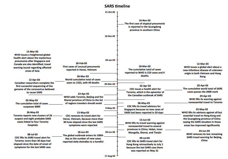
    [13] World Health Organization, Summary of Probable SARS Cases with Onset of Illness from 1 November 2002 to 31 July 2003, https://www.who.int/csr/sars/country/table2004_04_21/en/. Accessed 13 Oct 2020.
    [14] S. Riley, C. Fraser, C. A. Donnelly, A. C. Ghani, L. J. Abu-Raddad, A. J. Hedley, et al., Transmission Dynamics of the Etiological Agent of SARS in Hong Kong: Impact of Public Health Interventions, Science, 300 (2003), 1961-1966. doi: 10.1126/science.1086478
    [15] G. Chowell, P. W. Fenimore, M. A. Castillo-Garsow, C. C. Castillo-Chavez, SARS Outbreaks in Ontario, Hong Kong and Singapore: The Role of Diagnosis and Isolation as a Control Mechanism, J. Theor. Biol., 224 (2003), 1-8. doi: 10.1016/S0022-5193(03)00228-5
    [16] M. Lipsitch, T. Cohen, B. Cooper, J. M. Robins, S. Ma, L. James, et al., Transmission Dynamics and Control of Severe Acute Respiratory Syndrome, Science, 300 (2003), 1966-1970. doi: 10.1126/science.1086616
    [17] G. Zhou, G. Yan. Severe Acute Respiratory Syndrome Epidemic in Asia, Emerging Infect. Dis., 9 (2003), 1608-1610.
    [18] B. C. K. Choi, A. W. P. Pak. A Simple Approximate Mathematical Model to Predict the Number of Severe Acute Respiratory Syndrome Cases and Deaths, J. Epidemiology Community Health, 57 (2003), 831-835. doi: 10.1136/jech.57.10.831
    [19] L. O. Lloyd-Smith, A. P. Galvani, W. M. Getz, Curtailing Transmission of Severe Acute Respiratory Syndrome within a Community and Its Hospital, Proc. Royal Soc. B, 270, (2003), 1979-1989. doi: 10.1098/rspb.2003.2481
    [20] S. A. Eifan, I. Nour, A. Hanif, A. M. Zamzam, S. M. AlJohani, A Pandemic Risk Assessment of Middle East Respiratory Syndrome Coronavirus (MERS-CoV) in Saudi Arabia, Saudi J. Biol. Sci., 24 (2017), 1631-1638. doi: 10.1016/j.sjbs.2017.06.001
    [21] G. Chowell, F. Abdirizak, S. Lee, J. Lee, E. Jung, H. Nishiura, et al., Transmission Characteristics of MERS and SARS in the Healthcare Setting: A Comparative Study, BMC Med., 13 (2015), 210. doi: 10.1186/s12916-015-0450-0
    [22] C. Drosten, B. Meyer, M. A. Müller, V. M. Corman, M. Al-Masri, R. Hossain, et al., Transmission of MERS-coronavirus in household contacts, N. Engl. J. Med., 371 (2014), 828-835. doi: 10.1056/NEJMoa1405858
    [23] S. Cauchemez, C. Fraser, M. D. Van Kerkhove, C. A. Donnelly, S. Riley, A. Rambaut, et al., Middle East Respiratory Syndrome Coronavirus: Quantification of the Extent of the Epidemic, Surveillance Biases, and Transmissibility, Lancet Infect. Dis., 14 (2014), 50-56. doi: 10.1016/S1473-3099(13)70304-9
    [24] R. Breban, J. Riou, A. Fontanet, Interhuman Transmissibility of Middle East Respiratory Syndrome Coronavirus: Estimation of Pandemic Risk, Lancet, 382 (2013), 694-699. doi: 10.1016/S0140-6736(13)61492-0
    [25] H.-J. Chang, Estimation of Basic Reproduction Number of the Middle East Respiratory Syndrome Coronavirus (MERS-CoV) during the Outbreak in South Korea, 2015, BioMed. Eng. OnLine, 16 (2017), 79. doi: 10.1186/s12938-017-0370-7
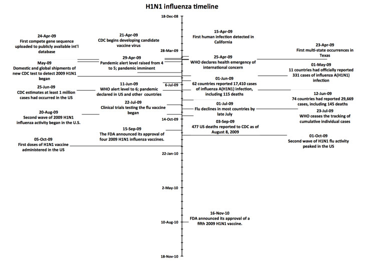
    [26] Centers for Disease Control, H1N1 Flu Pandemic Timeline. Centers for Disease Control and Prevention, https://www.cdc.gov/flu/pandemic-resources/2009-pandemic-timeline.html, Accessed 13 Oct 2020.
    [27] T. N. Jilani, R. T. Jamil, A. H. Siddiqui, H1N1 Influenza (Swine Flu). StatPearls, 2020, http://www.ncbi.nlm.nih.gov/books/NBK513241/ Accessed 13 Oct 2020.
    [28] Centers for Disease Control, 2009 H1N1 Pandemic (H1N1pdm09 virus), https://www.cdc.gov/flu/pandemic-resources/2009-h1n1-pandemic.html Accessed 13 Oct 2020.
    [29] M. G. Roberts, H. Nishiura, Early Estimation of the Reproduction Number in the Presence of Imported Cases: Pandemic Influenza H1N1-2009 in New Zealand, PLoS ONE, 6 (2011), e17835. doi: 10.1371/journal.pone.0017835
    [30] C. Fraser, C. A. Donnelly, S. Cauchemez, W. P. Hanage, M. D. Van Kerkhove, T. D. Hollingsworth, et al., Pandemic Potential of a Strain of Influenza A (H1N1): Early Findings, Science, 324 (2009), 1557-1561. doi: 10.1126/science.1176062
    [31] H. Nishiura, C. Castillo-Chavez, M. Safan M, G. Chowell, Transmission Potential of the New Influenza A(H1N1) Virus and Its Age-Specificity in Japan, Euro. Surveil., 14 (2009), 19227.
    [32] L. F. White, J. Wallinga, L. Finelli, C. Reed, S. Riley, M. Lipsitch, et al., Estimation of the Reproductive Number and the Serial Interval in Early Phase of the 2009 Influenza A/H1N1 Pandemic in the USA, Influenza Other Respir. Viruses, 3 (2009), 267-276. doi: 10.1111/j.1750-2659.2009.00106.x
    [33] L. C. Mostąo-Guidolin, C. S. Bowman, A. L. Greer, D. N. Fisman, S. M. Moghadas, Transmissibility of the 2009 H1N1 Pandemic in Remote and Isolated Canadian Communities: A Modelling Study, BMJ Open, 2 (2012), e001614. doi: 10.1136/bmjopen-2012-001614
    [34] M. Helferty, J. Vachon, J. Tarasuk, R. Rodin, J. Spika, L. Pelletier, Incidence of Hospital Admissions and Severe Outcomes during the First and Second Waves of Pandemic (H1N1) 2009, CMAJ, 182 (2010), 1981-1987. doi: 10.1503/cmaj.100746
    [35] O. T. Mytton, P. D. Rutter, M. Mak, E. A. Stanton, N. Sachedina, L. J. Donaldson, Mortality Due to Pandemic (H1N1) 2009 Influenza in England: A Comparison of the First and Second Waves, Epidemiol. Infect., 140 (2012), 1533-1541. doi: 10.1017/S0950268811001968
    [36] I. Dorigatti, S. Cauchemez, N. M. Ferguson, Increased Transmissibility Explains the Third Wave of Infection by the 2009 H1N1 Pandemic Virus in England, Proc. Natl. Acad. Sci. U.S.A., 110 (2013), 13422-13427. doi: 10.1073/pnas.1303117110
    [37] O. Sharomi, C. N. Podder, A. B. Gumel, S. M. Mahmud, E. Rubinstein, Modelling the Transmission Dynamics and Control of the Novel 2009 Swine Influenza (H1N1) Pandemic, Bull. Math. Biol., 73 (2011), 515-548. doi: 10.1007/s11538-010-9538-z
    [38] M. A. Jhung, D. Swerdlow, S. J. Olsen, D. Jernigan, M. Biggerstaff, L. Kamimoto, et al., Epidemiology of 2009 pandemic influenza A (H1N1) in the United States, Clin. Infect. Dis., 52 (2011), S13-S26. doi: 10.1093/cid/ciq008
    [39] M. D. Van Kerkhove, A. W. Mounts, S. Mall, K. A. Vandemaele, M. Chamberland, T. dos Santos, et al., Epidemiologic and virologic assessment of the 2009 influenza A (H1N1) pandemic on selected temperate countries in the Southern Hemisphere: Argentina, Australia, Chile, New Zealand and South Africa, Influenza Other Respir. Viruses, 5 (2011), e487-e498. doi: 10.1111/j.1750-2659.2011.00249.x
    [40] R. J. Smith?, Did we Eradicate SARS? Lessons Learned and the Way Forward, Am. J. Biomed. Sci. Res., 6 (2019), 001017.
    [41] R. M. Anderson, C. Fraser, A. C. Ghani, C. A. Donnelly, S. Riley, N. M. Ferguson, et al., Epidemiology, Transmission Dynamics and Control of SARS: The 2002-2003 Epidemic, Philos. Trans. R. Soc. Lond., B, Biol. Sci., 359 (2004), 1091-105. doi: 10.1098/rstb.2004.1490
    [42] S. Ruan, W. Wang, S. A. Levin, The Effect of Global Travel on the Spread of SARS, Math. Biosci. Eng., 3 (2006), 205-218. doi: 10.3934/mbe.2006.3.205
    [43] N. G. Becker, K. Glass, Z. Li, G. K. Aldis, Controlling Emerging Infectious Diseases like SARS, Math. Biosci., 193 (2005), 205-121. doi: 10.1016/j.mbs.2004.07.006
    [44] A. J. Kucharski, C. L. Althaus, The role of superspreading in Middle East respiratory syndrome coronavirus (MERS-CoV) transmission, Euro. Surveil. 20 (2015), 14-18.
    [45] S. Bernard-Stoecklin, B. Nikolay, A. Assiri, A. A. Saeed, P. K. Embarek, H. El Bushra, et al., Comparative Analysis of Eleven Healthcare-Associated Outbreaks of Middle East Respiratory Syndrome Coronavirus (Mers-Cov) from 2015 to 2017, Sci. Rep., 9 (2019), 1-9. doi: 10.1038/s41598-018-37186-2
    [46] S. Choi, E. Jung, B. Y. Choi, Y. J. Hur, M. Ki, High Reproduction Number of Middle East Respiratory Syndrome Coronavirus in Nosocomial Outbreaks: Mathematical Modelling in Saudi Arabia and South Korea, J. Hosp. Infect., 99 (2018), 162-168. doi: 10.1016/j.jhin.2017.09.017
    [47] T. Sardar, I. Ghosh, X. Rodó, J. Chattopadhyay, A Realistic Two-Strain Model for MERS-CoV Infection Uncovers the High Risk for Epidemic Propagation, PLOS Negl. Trop. Dis., 14 (2020), e0008065. doi: 10.1371/journal.pntd.0008065
    [48] M. S. Majumder, C. Rivers, E. Lofgren, D. Fisman. Estimation of MERS-Coronavirus Reproductive Number and Case Fatality Rate for the Spring 2014 Saudi Arabia Outbreak: Insights from Publicly Available Data, PLoS Currents, 6 (2014).
    [49] P. Poletti, M. Ajelli, S. Merler, The effect of risk perception on the 2009 H1N1 pandemic influenza dynamics, PLoS One, 6 (2011), e16460. doi: 10.1371/journal.pone.0016460
    [50] S. Tsukui, Case-Based Surveillance of Pandemic (H1N1) 2009 in Maebashi City, Japan, Jpn. J. Infect. Dis., 65 (2012), 132-137.
    [51] G. Chowell, S. Echevarria-Zuno, C. Viboud, L. Simonsen, J. Tamerius, M. A. Miller, et al., Characterizing the epidemiology of the 2009 influenza A/H1N1 pandemic in Mexico, PLoS Med., 8 (2011), e1000436. doi: 10.1371/journal.pmed.1000436
    [52] C. M. Rivers, E. T. Lofgren, M. Marathe, S. Eubank, B. L. Lewis, Modeling the impact of interventions on an epidemic of Ebola in Sierra Leone and Liberia, PLOS Currents Outbreaks, 6 (2014).
    [53] D. Fisman, E. Khoo, A. Tuite, Early epidemic dynamics of the West African 2014 Ebola outbreak: Estimates derived with a simple two-parameter model, PLoS Currents, 6 (2014).
    [54] C. Browne, H. Gulbudak, G. Webb, Modeling contact tracing in outbreaks with application to Ebola, J. Theor. Biol., 384 (2015), 33-49. doi: 10.1016/j.jtbi.2015.08.004
    [55] G. Webb, C. Browne, A model of the Ebola epidemics in West Africa incorporating age of infection, J. Biol. Dyn., 10 (2016), 18-30. doi: 10.1080/17513758.2015.1090632
    [56] T. S. Do, Y. S. Lee, Modeling the spread of Ebola. Osong Public Health and Research Perspectives, 7 (2016), 43-48. doi: 10.1016/j.phrp.2015.12.012
    [57] D. Salem, R. Smith?, A Mathematical Model of Ebola Virus Disease: Using Sensitivity Analysis to Determine Effective Intervention Targets, Proceedings of the SummerSim-SCSC 2016 conference, (2016), 16-23.
    [58] P. Bhandari, Analysis of Prediction Models in spread of Ebola Virus Disease, Thesis, Deakin University (2019).
    [59] T. C. Germann, K. Kadau, I. M. Longini, C. A. Macken, Mitigation strategies for pandemic influenza in the United States, Proc. Natl. Acad. Sci.U. S.A., 103 (2006), 5935-5940. doi: 10.1073/pnas.0601266103
    [60] J. T. Wu, B. J. Cowling, The use of mathematical models to inform influenza pandemic preparedness and response, Exp. Biol. Med., 236 (2011), 955-961. doi: 10.1258/ebm.2010.010271
    [61] S. S. Morse, J. A. Mazet, M. Woolhouse, C. R. Parrish, D. Carroll, W. B. Karesh, et al., Prediction and prevention of the next pandemic zoonosis, Lancet, 380 (2012), 1956-1965. doi: 10.1016/S0140-6736(12)61684-5
    [62] A. Huppert, G. Katriel, Mathematical modelling and prediction in infectious disease epidemiology, Clin. Microbiol. Infect., 19 (2013), 999-1005. doi: 10.1111/1469-0691.12308
    [63] P. Saunders-Hastings, B. Q. Hayes, R. Smith? D. Krewski. Modelling community-control strategies to protect hospital resources during an influenza pandemic in Ottawa, Canada, PloS One, 12 (2017), e0179315. doi: 10.1371/journal.pone.0174953
    [64] M. Valenciano, E. Kissling, J. M. Cohen, N. Oroszi, A. S. Barret, C. Rizzo, et al., Estimates of pandemic influenza vaccine effectiveness in Europe, 2009-2010: results of Influenza Monitoring Vaccine Effectiveness in Europe (I-MOVE) multicentre case-control study, PLoS Med., 8 (2011), e1000388. doi: 10.1371/journal.pmed.1000388
  • This article has been cited by:

    1. Serena Dipierro, Luca Lombardini, Partial differential equations from theory to applications: Dedicated to Alberto Farina, on the occasion of his 50th birthday, 2023, 5, 2640-3501, 1, 10.3934/mine.2023050
    2. Alessandra De Luca, Veronica Felli, Stefano Vita, Strong unique continuation and local asymptotics at the boundary for fractional elliptic equations, 2022, 400, 00018708, 108279, 10.1016/j.aim.2022.108279
    3. Alessandra De Luca, Veronica Felli, Stefano Vita, Unique Continuation from Conical Boundary Points for Fractional Equations, 2025, 57, 0036-1410, 907, 10.1137/24M1663193
  • Reader Comments
  • © 2020 the Author(s), licensee AIMS Press. This is an open access article distributed under the terms of the Creative Commons Attribution License (http://creativecommons.org/licenses/by/4.0)
通讯作者: 陈斌, bchen63@163.com
  • 1. 

    沈阳化工大学材料科学与工程学院 沈阳 110142

  1. 本站搜索
  2. 百度学术搜索
  3. 万方数据库搜索
  4. CNKI搜索

Metrics

Article views(15584) PDF downloads(199) Cited by(0)

Figures and Tables

Figures(4)

/

DownLoad:  Full-Size Img  PowerPoint
Return
Return

Catalog