Modal identification of a high-rise building subjected to a landfall typhoon via both deterministic and Bayesian methods

Yuncheng He; Zhen Liu; Zhi Li; Jiurong Wu; Jiyang Fu; Yuncheng He; Zhen Liu; Zhi Li; Jiurong Wu; Jiyang Fu

doi:10.3934/mbe.2019359

Mathematical Biosciences and Engineering

2019, Volume 16, Issue 6: 7155-7176. doi: 10.3934/mbe.2019359

Previous Article Next Article

Research article Special Issues

Modal identification of a high-rise building subjected to a landfall typhoon via both deterministic and Bayesian methods

Joint Research Center for Engineering Structure Disaster Prevention and Control, Guangzhou University Guangdong 510006, China

Received: 30 April 2019 Accepted: 28 July 2019 Published: 07 August 2019

Modal identification involves primarily the determination of natural frequencies, damping ratios, mode shapes of a dynamic system, etc. It is usually regarded as an essential task in a wide branch of structural dynamics and civil engineering, such as structural vibration control and damage identification of buildings or bridges. There are many modal identification techniques. Basically, these techniques can be categorized into two groups: deterministic methods and Bayesian approaches. The first group can be used to provide deterministic (or optimal) estimations of modal parameters, but they are unable to quantify the estimation uncertainties. The second group is based on a usage of the Bayesian framework. Compared to the first group, the second group of methods has a typical merit of being able to offer uncertainty information of identified parameters, which is of great interests, or even necessary, for some follow-up studies. In this paper, both a deterministic method, i.e., a combination of spectral analysis, filtering and Random Decrement Technique (RDT), and a Bayesian method, i.e., Bayesian Spectral Density Approach (BSDA), are exploited to experimentally identify the modal parameters of a 303 m high-rise building that was subjected to a landfall typhoon. The validity and efficiency of each method is verified by comparing the two kinds of results. Meanwhile, the identified modal parameters are used for the serviceability assessment of this high-rise building against some frequency-specific criteria.
- modal identification,
- Bayesian approach,
- deterministic method,
- high-rise building,
- typhoon
Citation: Yuncheng He, Zhen Liu, Zhi Li, Jiurong Wu, Jiyang Fu. Modal identification of a high-rise building subjected to a landfall typhoon via both deterministic and Bayesian methods[J]. Mathematical Biosciences and Engineering, 2019, 16(6): 7155-7176. doi: 10.3934/mbe.2019359

Related Papers:

Abstract

Modal identification involves primarily the determination of natural frequencies, damping ratios, mode shapes of a dynamic system, etc. It is usually regarded as an essential task in a wide branch of structural dynamics and civil engineering, such as structural vibration control and damage identification of buildings or bridges. There are many modal identification techniques. Basically, these techniques can be categorized into two groups: deterministic methods and Bayesian approaches. The first group can be used to provide deterministic (or optimal) estimations of modal parameters, but they are unable to quantify the estimation uncertainties. The second group is based on a usage of the Bayesian framework. Compared to the first group, the second group of methods has a typical merit of being able to offer uncertainty information of identified parameters, which is of great interests, or even necessary, for some follow-up studies. In this paper, both a deterministic method, i.e., a combination of spectral analysis, filtering and Random Decrement Technique (RDT), and a Bayesian method, i.e., Bayesian Spectral Density Approach (BSDA), are exploited to experimentally identify the modal parameters of a 303 m high-rise building that was subjected to a landfall typhoon. The validity and efficiency of each method is verified by comparing the two kinds of results. Meanwhile, the identified modal parameters are used for the serviceability assessment of this high-rise building against some frequency-specific criteria.

References

[1]	Q. S. Li, L. H. Zhi, A.Y. Tuan, et al., Dynamic behavior of Taipei 101 tower: Field Measurement and Numerical Analysis, J. Struct. Eng., 137 (2010), 143–155.
[2]	W. Shi, J. Shan and X. Lu, Modal identification of Shanghai World Financial Center both from free and ambient vibration response, Eng. Struct., 36 (2012), 14–26.
[3]	H. Akaike, Power spectrum estimation through autoregressive model fitting, Ann. I. Stat. Math., 21 (1969), 407–419.
[4]	H. A. Cole Jr, On-line failure detection and damping measurement of aerospace structures by random decrement signatures, NASA Cr-2205: Washington, DC, USA, (1973).
[5]	F. Nasser, Z. Li, N. Martin, et al., An automatic approach towards modal parameter estimation for high-rise buildings of multicomponent signals under ambient excitations via filter-free Random Decrement Technique, Mech. Syst. Signal Proc., 70(2016), 821–831.
[6]	S. R. Ibrahim and E. C. Mikulcik, A time domain modal vibration test technique, Shock Vib. Bull., 43 (1973), 21–37.
[7]	J. N. Juang and R. S. Pappa, An eigensystem realization algorithm for modal parameter identification and model reduction, JGCD., 8 (1985), 620–627.
[8]	B. Peeters and G. De Roeck, Reference-based stochastic subspace identification for output-only modal analysis, Mech. Syst. Signal Proc., 13 (1999), 855-878.
[9]	G. H. J. Ill, T. G. Carrie and J. P. Lauffer, The Natural Excitation Technique (NExT) for Modal Parameter Extraction from Operating Wind Turbines, NASA STI/Rec on Technical Report N., 93 (1993), 260–277.
[10]	D. L. Brown, R. J. Allemang, R. Zimmerman, et al., Parameter Estimation Techniques for Modal Analysis, SAE transactions., (1979), 828–846.
[11]	J. S. Bendat and A. G. Piersol, Engineering applications of correlation and spectral analysis, New York, Wiley-Interscience., (1993), 315.
[12]	Y. He, Q. Li, H. Zhu, et al., Monitoring of structural modal parameters and dynamic responses of a 600m-high skyscraper during a typhoon, Struct. Des. Tall Spec. Build., 27(2018), 1456.
[13]	R. Brincker, L. Zhang and P. Andersen, Modal identification from ambient responses using frequency domain decomposition, Process of the 18th International Modal Analysis Conference, San Antonio, Texas., (2000), 625–630.
[14]	I. Daubechies, The wavelet transform, time-frequency localization and signal analysis, IEEE Trans. Inf. Theory., 36 (1990), 961–1005.
[15]	N. E. Huang, Z. Shen, S. R. Long, et al., The empirical mode decomposition method and the Hilbert spectrum for non-stationary time series analysis, Proc. Roy. Soc. London., 454 (1998), 903–995.
[16]	J. F. Clinton, S. C. Bradford, T. H. Heaton, et al., The observed wander of the natural frequencies in a structure, Bull Seismol Soc Am., 96 (2006), 237–257.
[17]	R. D. Nayeri, S. F. Masri, R. G. Ghanem, et al., A novel approach for the structural identification and monitoring of a full-scale 17-story building based on ambient vibration measurements, Smart Mater. Struct., 17 (2008), 1–19.
[18]	A. Mikael, P. Gueguen, P. Y. Bard, et al., The analysis of long-term frequency and damping wandering in buildings using the Random Decrement Technique, Bull Seismol Soc Am., 103 (2013), 236–246.
[19]	Z. C. Yang, Y. H. Huang, A. R. Liu, et al., Nonlinear in-plane buckling of fixed shallow functionally graded grapheme reinforced composite arches subjected to mechanical and thermal loading, Appl. Math. Model., 70 (2019), 315–327.
[20]	J. L. Beck and L S. Katafygiotis, Updating Models and Their Uncertainties. I: Bayesian Statistical Framework, J. Eng. Mech., 124 (1998), 455–461.
[21]	L. S. Katafygiotis, C. Papadimitriou and H. F. Lam, A probabilistic approach to structural model updating, Soil Dyn. Earthq. Eng., 17 (1998), 495–507.
[22]	L. S. Katafygiotis and K. V. Yuen, Bayes spectral density approach for modal updating using ambient data, Earthq. Eng. Struct. Dyn., 30 (2001), 1103–1123.
[23]	K. V. Yuen and L. S. Katafygiotis, Bayesian Modal Updating Using Complete Input and Incomplete Response Noisy Measurements, J. Eng. Mech., 128 (2002), 340–350.
[24]	S. K. Au, Fast Bayesian FFT method for ambient modal identification with separated modes, J. Eng. Mech., 137 (2011), 214–226.
[25]	S. K. Au, Connecting Bayesian and frequentist quantification of parameter uncertainty in system identification, Mech. Syst. Signal Proc., 29 (2012), 328–342.
[26]	F. L. Zhang, H. B. Xiong, W. X. Shi, et al., Structural health monitoring of Shanghai Tower during different stages using a Bayesian approach, Struct. Control. Health Monit., 23 (2016), 1366–1384.
[27]	X. Li and Q. S. Li, Observations of typhoon effects on a high-rise building and verification of wind tunnel predictions, J. Wind Eng. Ind. Aerodyn., 84 (2019), 174–184.
[28]	S. C. Kuok and K. V. Yuen, Structural health monitoring of Canton Tower using Bayesian framework, Smart. Struct. Syst., 10 (2012), 375–391.
[29]	Z. Li, M. Q. Feng, L. Luo, et al., Statistical analysis of modal parameters of a suspension bridge based on Bayesian spectral density approach and SHM data, Mech. Syst. Signal Proc., 98 (2018), 352–367.
[30]	A. Alkan and M. K. Kiymik, Comparison of AR and Welch Methods in Epileptic Seizure Detection, J. Med. Syst., 30 (2006), 413–419.
[31]	A. Alkan and A. S. Yilmaz, Frequency domain analysis of power system transients using Welch and Yule-Walker AR methods, Energy Conv. Manag., 48 (2007), 2129–2135.
[32]	W. Shi, J. Shan and X. Lu, Modal identification of Shanghai World Financial Center both from free and ambient vibration response, Eng. Struct., 36 (2012), 14–26.
[33]	K. V. Yuen and J. L. Beck, Updating properties of nonlinear dynamical systems with uncertain input, J. Eng. Mech., 129 (2003), 9–20.
[34]	P. R. Krishnaiah, Some recent developments on complex multivariate distributions, J. Multivariate Anal., 6 (1976), 1–30.
[35]	K. V. Yuen, Bayesian methods for structural dynamics and civil engineering, Wiley: New York., 2010.
[36]	Y. C. He and Q. S. Li, Dynamic responses of a 492-m-high tall building with active tuned mass damping system during a typhoon, Struct. Control. Health Monit., 21(2014), 705–720.
[37]	Z. Li, J. Y. Fu, H. J. Mao, et al., Modal identification of civil structures via covariance-driven stochastic subspace method, Math. Biosci. Eng., 16 (2019), 5709–5728.
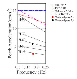
[38]	International Standardization Organization (ISO), Bases for Design of Structures-Serviceability of Buildings and Walkways against Vibrations, ISO 10137 (2^nd Ed.), Geneva., 2007.
[39]	W. H. Melbourne, Probability distributions associated with the wind loading structures, Civ. Eng. Trans. Inst. Eng. Aust. CE19., 1 (1977), 58–67.
[40]	W. H. Melbourne and T. R. Palmer, Accelerations and comfort criteria for buildings undergoing complex motions, J. Wind Eng. Ind. Aerodyn., 44 (1992), 105–116.
[41]	Y. Tamura, H. Kawai, Y. Uematsu, et al., Documents for wind resistant design of buildings in Japan. Workshop on Regional Harmonization of Wind Loading and Wind Environmental Specifications in Asia-Pacific Economies (APEC-WW), (2004), 61–84.
[42]	AL-GBV, Guidelines for the evaluation habitability to building vibration, AIJE-V001-2004, Tokyo, Japan, (2004).
[43]	JGJ 3-2010. Technical specification for concrete structures of tall building, China Building Industry Press: Beijing, (2010).

Reader Comments

Your name:*

Email:*
© 2019 the Author(s), licensee AIMS Press. This is an open access article distributed under the terms of the Creative Commons Attribution License (http://creativecommons.org/licenses/by/4.0)